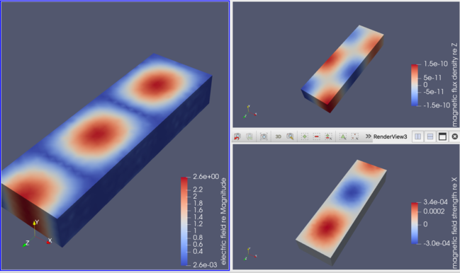
矩形導波管解析 ( Vectorial Helmholtz Equation )
矩形導波管を例として、電磁波のFEM解析手法について述べる.
電磁波解析には、時系列的な解析手法(FDTD)と周波数解析(単一周波数の振幅分布を求める)手法がある.
波動解析全般において、勿論、波動方程式が成立する. Maxwell 方程式も例外ではない.波動方程式の Fourier 変換は、Helmholtz 方程式となる.
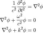
周波数空間における波動伝搬の解析は、Helmholtz 方程式を解けば良い. Helmholtz 方程式は、 Poisson 方程式の非線形解析型であるので、FEMを用いて解ける.
上記、スカラー関数での議論は、電磁波の3次元ベクトルの場合にも適用できる.電磁波の場合、前項で示したベクトル型 Helmholtz 方程式( Vectorial Helmholtz Equation )となる.
問題設定 / メッシュ / 境界条件
問題設定
矩形導波管( 矩形断面長さ: a ,b 、長さ L )内を伝搬する電磁波を考える.
電磁波の周波数は、
 .
.解析対象は TE10 モード
パラメータ設定
矩形断面
 を考えてみる. ( 典型例として、
  としている.)
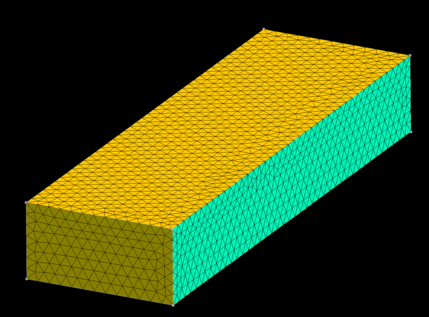
メッシュ
メッシュ生成用スクリプトファイルを以下に示す.
 1import os, sys
 2import numpy         as np
 3import gmsh_api.gmsh as gmsh
 4
 5# ------------------------------------------------- #
 6# --- [1] initialization of the gmsh            --- #
 7# ------------------------------------------------- #
 8gmsh.initialize()
 9gmsh.option.setNumber( "General.Terminal", 1 )
10gmsh.model.add( "model" )
11
12# ------------------------------------------------- #
13# --- [2] initialize settings                   --- #
14# ------------------------------------------------- #
15ptsDim , lineDim , surfDim , voluDim  =  0,  1,  2, 3
16pts    , line    , surf    , volu     = {}, {}, {}, {}
17ptsPhys, linePhys, surfPhys, voluPhys = {}, {}, {}, {}
18x_, y_, z_, lc_, tag_                 = 0, 1, 2, 3, 4
19
20# ------------------------------------------------- #
21# --- [3] Modeling                              --- #
22# ------------------------------------------------- #
23
24import nkGmshRoutines.generate__quadShape as gqs
25
26lc_inner     = 0.0300
27
28wg_a         = 0.3810
29wg_b         = 0.1905
30wg_L         = 1.2138478633282366
31
32x1_wg_i      = [  0.0,   0.0,  0.0 ]
33x2_wg_i      = [ wg_a,   0.0,  0.0 ]
34x3_wg_i      = [ wg_a,  wg_b,  0.0 ]
35x4_wg_i      = [  0.0,  wg_b,  0.0 ]
36
37ex_delta     = [  0.0,   0.0, wg_L ]
38
39ret1         = gqs.generate__quadShape( lc=lc_inner, defineVolu=True, extrude_delta=ex_delta, \
40                                        x1=x1_wg_i , x2=x2_wg_i, \
41                                        x3=x3_wg_i , x4=x4_wg_i, recombine=False )
42
43
44# ------------------------------------------------- #
45# --- [4] attribute physical number             --- #
46# ------------------------------------------------- #
47
48import nkGmshRoutines.load__physNumTable as pnt
49pnt.load__physNumTable( inpFile="physNumTable.dat", line=line, surf=surf )
50
51
52# ------------------------------------------------- #
53# --- [5] post process                          --- #
54# ------------------------------------------------- #
55gmsh.model.occ.synchronize()
56gmsh.model.mesh.generate(3)
57gmsh.write( "model.geo_unrolled" )
58gmsh.write( "model.msh" )
59gmsh.finalize()
60
用いたメッシュを以下に示す.
境界条件
境界条件としては、電磁波の入射境界 ( -z 境界 )と出射境界 ( +z 境界 )、及び、導体境界からなる.
elmer 入力ファイル ( .sif ファイル )
elmer用の入力ファイルを以下に示す.
  1
  2! ========================================================= !
  3! ===  waveguide simulation                             === !
  4! ========================================================= !
  5
  6! ------------------------------------------------- !
  7! --- [1] Global Simulation Settings            --- !
  8! ------------------------------------------------- !
  9
 10Check Keywords "Warn"
 11
 12Header
 13  Mesh DB "." "model"
 14  Include Path ""
 15  Results Directory ""
 16End
 17
 18Simulation
 19  Coordinate System           = String "Cartesian"
 20  Coordinate Mapping(3)       = 1 2 3
 21
 22  Simulation Type             = Steady
 23  Steady State Max Iterations = Integer 1
 24  Output Intervals            = Integer 1
 25  Timestepping Method         = BDF
 26  BDF Order                   = Integer 1
 27
 28  Solver Input File           = "waveguide.sif"
 29  Output File                 = "waveguide.dat"
 30  Post File                   = "vectorhelmholtz.vtu"
 31End
 32
 33Constants
 34  ! Do NOT write down - permeability - an error somehow occurs...!!!
 35  ! Permeability of Vacuum      = 1.2566e-06
 36  ! Permittivity of Vacuum      = 8.8542e-12
 37End
 38
 39! ------------------------------------------------- !
 40! --- [2] Body & Material Settings              --- !
 41! ------------------------------------------------- !
 42
 43Body 1
 44  Target Bodies(1)       = 301
 45  Name                   = "wavepath"
 46
 47  Equation               = 1
 48  Material               = 1
 49  Initial Condition      = 1
 50End
 51
 52Material 1
 53  Name                   = "Air"
 54  Electric Conductivity  = 0.0
 55  Relative Permittivity  = 1.0
 56  Relative Permeability  = 1.0
 57End
 58
 59
 60! ------------------------------------------------- !
 61! --- [3] Equation & Solver Settings            --- !
 62! ------------------------------------------------- !
 63
 64$ freq  = 5.001e8
 65$ wg_a  = 0.3810
 66$ wg_b  = 0.1905
 67$ wg_L  = 1.2138478633282366
 68$ wAmp  = 1.0
 69
 70$ mmode = 1
 71$ nmode = 0
 72$ epsil = 8.854e-12
 73$ mu    = 4.0*pi*10^-7
 74$ c0    = 1.0 / sqrt( epsil * mu )
 75$ omega = 2.0 * pi * freq
 76$ k0    = omega / c0
 77$ kx    = mmode * pi / wg_a
 78$ ky    = nmode * pi / wg_b
 79$ kc    = sqrt( kx^2 + ky^2 )
 80$ beta0 = sqrt( k0^2 - kc^2 )
 81$ Acoef = omega * mu * kx * wAmp / kc^2
 82$ sigma = 5.e3
 83$ Zp_m  = sqrt( 0.5 * mu * omega / sigma )
 84$ alp_m = omega * mu / Zp_m
 85! alpha_for_metal = -i / ( 1 - i ) * alp_m = ( 1-i ) / 2 * alp_m ...> set this value as B.C.
 86
 87
 88Equation 1
 89  Name                                     = "waveguide_EMpath"
 90  Active Solvers(3)                        = 1 2 3
 91  Angular Frequency                        = Real $omega
 92End
 93
 94
 95Solver 1
 96  Equation                                 = "VectorHelmholtzEquation"
 97  Procedure                                = "VectorHelmholtz" "VectorHelmholtzSolver"
 98  Variable                                 = E[E re:1 E im:1]
 99  Exec Solver                              = String "Always"
100
101  Use Piola Transform                      = Logical True
102  Optimize Bandwidth                       = Logical True
103  Linear System Symmetric                  = Logical False
104  Linear System Scaling                    = Logical True
105  Linear System Solver                     = String "Iterative"
106  ! -- Method :: ( BiCGStabl / gmres ) -- !
107  Linear System Iterative Method           = String "gmres" ! or "BiCGStabl"
108  ! Linear System Iterative Method           = String "BiCGStabl" ! or "gmres"
109  ! BiCGstabl polynomial degree              = Integer 4
110
111  Steady State Convergence Tolerance       = Real 1.0e-9
112
113  Linear System Preconditioning            = String "vanka"
114  Linear System ILUT Tolerance             = Real    3.0e-3
115  Linear System Max Iterations             = Integer 5000
116  Linear System Convergence Tolerance      = Real    1.0e-9
117  Linear System Abort Not Converged        = Logical False
118  Linear System Residual Output            = Integer 8
119  Linear System Preconditioning Damp Coefficient    = Real 0.0
120  Linear System Preconditioning Damp Coefficient im = Real 1.0
121
122End
123
124
125Solver 2
126  Equation                                 = "calcFields"
127  Procedure                                = "VectorHelmholtz" "VectorHelmholtzCalcFields"
128  ! Field Variable                           = String "E"
129  Exec Solver                              = String "Always"
130  Use Piola Transform                      = Logical True
131  Optimize Bandwidth                       = Logical False ! "True"
132  Linear System Symmetric                  = Logical False
133  Linear System Scaling                    = Logical True
134  Linear System Solver                     = String "Iterative"
135  Linear System Iterative Method           = String "BiCGStabl" ! "CG"
136  BiCGstabl polynomial degree              = Integer 4
137
138  Calculate Elemental Fields               = Logical False
139  Calculate Magnetic Field Strength        = Logical True
140  Calculate Electric Field                 = Logical True
141  Calculate Poynting Vector                = Logical True
142  Calculate Magnetic Flux Density          = Logical True
143  Calculate Div of Poynting Vector         = Logical True
144
145  Steady State Convergence Tolerance       = 1.0e-9
146  Exported Variable 1                      = -dofs 3 Eref_re
147
148  Linear System Preconditioning            = String "None"
149  Linear System ILUT Tolerance             = Real    1e-5
150  Linear System Max Iterations             = Integer 5000
151  Linear System Convergence Tolerance      = Real    1.0e-9
152  Linear System Abort Not Converged        = Logical False
153  Linear System Residual Output            = Integer 10
154  Linear System Preconditioning Damp Coefficient    = Real 0.0
155  Linear System Preconditioning Damp Coefficient im = Real 1.0
156
157End
158
159
160Solver 3
161  Equation  = "SaveScalars"
162  Procedure = "SaveData" "SaveScalars"
163  FileName  = "dat/waveguide_scalars.dat"
164End
165
166
167! ------------------------------------------------- !
168! --- [4] Body Forces / Initial Conditions      --- !
169! ------------------------------------------------- !
170
171Initial Condition 1
172  Eref_re 1 = Real MATC "0.0"
173  Eref_re 2 = Variable coordinate 1, coordinate 3
174         Real MATC "sin(kx*tx(0))*( sin( beta0*tx(1) ) - sin( -beta0*tx(1)+2.0*beta0*wg_L) )"
175  Eref_re 3 = Real MATC "0.0"
176
177  ! Eref_re 2 = Variable coordinate 1, coordinate 3
178  ! Real MATC "( -1.0 )*Acoef*sin( kx*tx(0) )*sin( beta0*tx(1) )"
179
180End
181
182
183! ------------------------------------------------- !
184! --- [5] Boundary Conditions                   --- !
185! ------------------------------------------------- !
186
187Boundary Condition 1
188
189  Target Boundaries(1)          = 201
190  Name                          = "inport"
191
192  ! ------------------------------------ !
193  ! -- Port Feed condition            -- !
194  ! ------------------------------------ !
195  ! -- alpha = i \beta                -- !
196  ! -- g = 2 i \beta * ( n x E ) x n  -- !
197  ! ------------------------------------ !
198  Electric Robin Coefficient    = Real $ 0.0
199  Electric Robin Coefficient im = Real $ beta0
200  Magnetic Boundary Load 2      = Variable Coordinate 1
201      Real MATC "-2.0*beta0*k0/kc*sin(kx*tx)"
202      ! Real MATC "(-2.0)*beta0*Acoef*sin(kx*tx)"
203
204End
205
206
207Boundary Condition 2
208
209  Target Boundaries(1)          = 202
210  Name                          = "outport"
211
212  ! ------------------------------------ !
213  ! -- PEC condition                  -- !
214  ! ------------------------------------ !
215  ! -- perfect conductor ( nxE = 0 )  -- !
216  ! --  E re {e} = 0.0                -- !
217  ! --  E im {e} = 0.0                -- !
218  ! ------------------------------------ !
219  ! E re {e} = 0.0
220  ! E im {e} = 0.0
221
222  ! ------------------------------------ !
223  ! -- Impedance condition            -- !
224  ! ------------------------------------ !
225  ! -- alpha = i \beta                -- !
226  ! -- g = 2 i \beta * ( n x E ) x n  -- !
227  ! ------------------------------------ !
228  ! Electric Robin Coefficient    = Real $ (  0.5 ) * alp_m
229  ! Electric Robin Coefficient im = Real $ ( -0.5 ) * alp_m
230  ! Magnetic Boundary Load 2      = Real $ 0.0
231  ! Magnetic Boundary Load 2 im   = Real $ 0.0
232
233
234  ! ------------------------------------ !
235  ! -- Neumann condition              -- !
236  ! ------------------------------------ !
237  ! -- alpha = 0.0                    -- !
238  ! -- g     = 0.0                    -- !
239  ! ------------------------------------ !
240  Electric Robin Coefficient    = Real $ 0.0
241  Electric Robin Coefficient im = Real $ 0.0
242  Magnetic Boundary Load 2      = Real $ 0.0
243  Magnetic Boundary Load 2 im   = Real $ 0.0
244
245End
246
247
248Boundary Condition 3
249
250  Target Boundaries(1)          = 203
251  Name                          = "sidewall"
252
253  ! ------------------------------------ !
254  ! -- PEC condition                  -- !
255  ! ------------------------------------ !
256  ! -- perfect conductor ( nxE = 0 )  -- !
257  ! --  E re {e} = 0.0                -- !
258  ! --  E im {e} = 0.0                -- !
259  ! ------------------------------------ !
260  E re {e} = 0.0
261  E im {e} = 0.0
262
263  ! ------------------------------------ !
264  ! -- Impedance condition            -- !
265  ! ------------------------------------ !
266  ! -- alpha = i \beta                -- !
267  ! -- g = 2 i \beta * ( n x E ) x n  -- !
268  ! ------------------------------------ !
269  ! Electric Robin Coefficient    = Real $ (  0.5 ) * alp_m
270  ! Electric Robin Coefficient im = Real $ ( -0.5 ) * alp_m
271  ! Magnetic Boundary Load 2      = Real $ 0.0
272  ! Magnetic Boundary Load 2 im   = Real $ 0.0
273
274
275  ! ------------------------------------ !
276  ! -- Neumann condition              -- !
277  ! ------------------------------------ !
278  ! -- alpha = 0.0                    -- !
279  ! -- g     = 0.0                    -- !
280  ! ------------------------------------ !
281  ! Electric Robin Coefficient    = Real $ 0.0
282  ! Electric Robin Coefficient im = Real $ 0.0
283  ! Magnetic Boundary Load 2      = Real $ 0.0
284  ! Magnetic Boundary Load 2 im   = Real $ 0.0
285
286End
287
重要命令は、以下の通りである.
(l.33-37) constants 内で自然な真空の透磁率・誘電率を指定してはいけない.何故かはわからないが、バグが生じてしまい、正しく計算できなくなる.
(l.64-85) パラメータ設定. $記号を用いて、elmer内部で変数を定義することができる.
(l.91) 解析対象とする角周波数.
(l.97,l.127) VectorHelmholtzソルバーを用いるという指示文.
(l.171-180) 比較対象とする解析解を initial condition として定義.内部では変数が用いられないからこの変数は変化しない.
(l.187-204) inport (風上側境界の電磁場指定).
 として、境界面での電場分布を与える.
(l.207-245) outport ( 風下側境界の電磁場指定 ).
 として、Neumann 境界条件を課す.
(l.248-286) 導波管壁の境界条件指定.
 として、 Dirichlet 境界条件を課す.