直方体中の熱伝導¶

シミュレーション名 :: heatConduction__in_a_bar_XYZ3D

シミュレーション体系¶

基本方程式は熱輸送方程式 ( Heat Equation )
シミュレーション対象は直方体 ( 10 [cm] x 10 [cm] x 100 [cm] )
一端を固定温度条件( 373.15 [K] = 100[℃] )、もう一端は自由境界条件（指定なし）
材質は銅 ( 熱伝導率：398 [W/mK]、比熱：379 [J/KgK]、8960 [kg/m3] )

メッシュ¶

メッシュ生成スクリプト ( mesh.py )

mesh.py ( heatConduction__in_a_bar_XYZ3D )¶

import numpy as np
import os, sys
import gmsh
import nkGmshRoutines.geometrize__fromTable as gft
import nkGmshRoutines.load__dimtags         as ldt

# ========================================================= #
# ===   実行部                                          === #
# ========================================================= #

if ( __name__=="__main__" ):

    # ------------------------------------------------- #
    # --- [1] initialization of the gmsh            --- #
    # ------------------------------------------------- #
    gmsh.initialize()
    gmsh.option.setNumber( "General.Terminal", 1 )
    gmsh.option.setNumber( "Mesh.Algorithm"  , 5 )
    gmsh.option.setNumber( "Mesh.Algorithm3D", 4 )
    gmsh.option.setNumber( "Mesh.SubdivisionAlgorithm", 0 )
    gmsh.model.add( "model" )
    
    # ------------------------------------------------- #
    # --- [2] Modeling                              --- #
    # ------------------------------------------------- #
    dimtags = {}
    inpFile = "dat/geometry.conf"
    dimtags = gft.geometrize__fromTable( inpFile=inpFile )
    inpFile = "dat/boundary.json"
    dimtags = ldt.load__dimtags( inpFile=inpFile, dimtags=dimtags )
    print( dimtags )
    
    gmsh.model.occ.synchronize()

    # ------------------------------------------------- #
    # --- [3] Mesh settings                         --- #
    # ------------------------------------------------- #
    mesh_from_config = True          # from nkGMshRoutines/test/mesh.conf, phys.conf
    uniform_size     = 0.010
    if ( mesh_from_config ):
        meshFile = "dat/mesh.conf"
        physFile = "dat/phys.conf"
        import nkGmshRoutines.assign__meshsize as ams
        meshes = ams.assign__meshsize( meshFile=meshFile, physFile=physFile, dimtags=dimtags )
    else:
        import nkGmshRoutines.assign__meshsize as ams
        meshes = ams.assign__meshsize( uniform=uniform_size, dimtags=dimtags )

    # ------------------------------------------------- #
    # --- [4] post process                          --- #
    # ------------------------------------------------- #
    gmsh.model.occ.synchronize()
    gmsh.model.mesh.generate(3)
    gmsh.write( "msh/model.msh" )
    gmsh.finalize()

geometry.conf

geometry.conf ( heatConduction__in_a_bar_XYZ3D )¶

# <define> @cube.wx   = 0.10
# <define> @cube.wy   = 0.10
# <define> @cube.wz   = 0.50

# <define> @cube.xMin = ( -0.5 ) * @cube.wx
# <define> @cube.yMin = ( -0.5 ) * @cube.wy
# <define> @cube.zMin = 0.0

# <names> key   geometry_type   centering  xc yc zc wx wy wz 
cube.01 cube False @cube.xMin @cube.yMin @cube.zMin @cube.wx @cube.wy @cube.wz

boundary.json

boundary.json ( heatConduction__in_a_bar_XYZ3D )¶

{"end.01": [[2, 5]], "end.02": [[2, 6]] }

phys.conf

phys.conf ( heatConduction__in_a_bar_XYZ3D )¶

# <names> key	type		dimtags_keys			physNum
cube.01		volu		[cube.01]			301
end.01		surf		[end.01]			201
end.02		surf		[end.02]			202

mesh.conf

mesh.conf ( heatConduction__in_a_bar_XYZ3D )¶

# <names> key	physNum	  meshType    resolution1	resolution2	evaluation
cube.01	  	301	  constant    0.010		-		-
end.01		201	  constant    0.0		-		-
end.02		202	  constant    0.0		-		-

生成したメッシュを次に示す．

Elmer シミュレーションファイル¶

シミュレーションファイル ( ns.sif )を以下に示す．

heat.sif ( heatConduction__in_a_bar_XYZ3D )¶

include "./msh/model/mesh.names"

Header
  CHECK KEYWORDS    Warn
  Mesh DB           "." "msh/model"
  Include Path      ""
  Results Directory "out/"
End


Simulation
  Max Output Level                         = 3
  Coordinate System                        = string "Cartesian"
  Coordinate Mapping(3)                    = 1 2 3

  Simulation Type                          = "Transient"
  TimeStepping Method                      = BDF
  BDF Order                                = 2
  Timestep sizes(1)                        = 20.0
  Timestep Intervals(1)                    = 50

  Steady State Max Iterations              = 1
End


Constants
  Stefan Boltzmann                         = 5.6703e-8  !!  -- [ W / m^2 K^4 ] --  !!
End


Solver 1
  Equation                                 = "HeatEquations"
  Procedure                                = "HeatSolve" "HeatSolver"
  Variable                                 = "Temperature"
  Exec Solver                              = "Always"
  Stabilize                                = True
  Bubbles                                  = False
  Optimize Bandwidth                       = True
  Steady State Convergence Tolerance       = 1.0e-5
  Nonlinear System Convergence Tolerance   = 1.0e-3
  Nonlinear System Max Iterations          = 1
  Nonlinear System Newton After Iterations = 3
  Nonlinear System Newton After Tolerance  = 1.0e-3
  Nonlinear System Relaxation Factor       = 1
  Linear System Solver                     = Iterative
  Linear System Iterative Method           = BiCGStab
  Linear System Max Iterations             = 500
  Linear System Convergence Tolerance      = 1.0e-10
  BiCGstabl polynomial degree              = 2
  Linear System Preconditioning            = ILU0
  Linear System ILUT Tolerance             = 1.0e-3
  Linear System Abort Not Converged        = False
  Linear System Residual Output            = 20
  Linear System Precondition Recompute     = 1
End


Solver 2
  Exec Solver                              = after saving
  Equation                                 = "Result output"
  Procedure                                = "ResultOutputSolve" "ResultOutputSolver"
  Output File Name                         = "heat"
  Vtu Format                               = Logical True
  Binary Output                            = Logical True
  Scalar Field 1                           = String temperature
End


Body 1
  Name                                     = "cube"
  Target Bodies(1)                         = $cube.01
  Equation                                 = 1
  Material                                 = 1
  Initial Condition                        = 1
End


Equation 1
  Name                                     = "ThermalConduction"
  Active Solvers(2)                        = 1 2
End


Material 1
  Name                                     = "Cupper" 
  Heat Conductivity                        = 398.0    !! W/m.K
  Heat Capacity                            = 379.0    !! J/kg.K
  Reference Temperature                    = 293.0    !! K
  Density                                  = 8.96e+3  !! kg/m3 
End


Initial Condition 1
  Name                                     = "cube.initial"
  temperature                              = 293.15   !! =  20 degree
End                                      

Boundary Condition 1
  Name                                     = ""
  Target Boundaries(1)                     = $end.01
  temperature                              = 373.15   !! = 100 degree
End

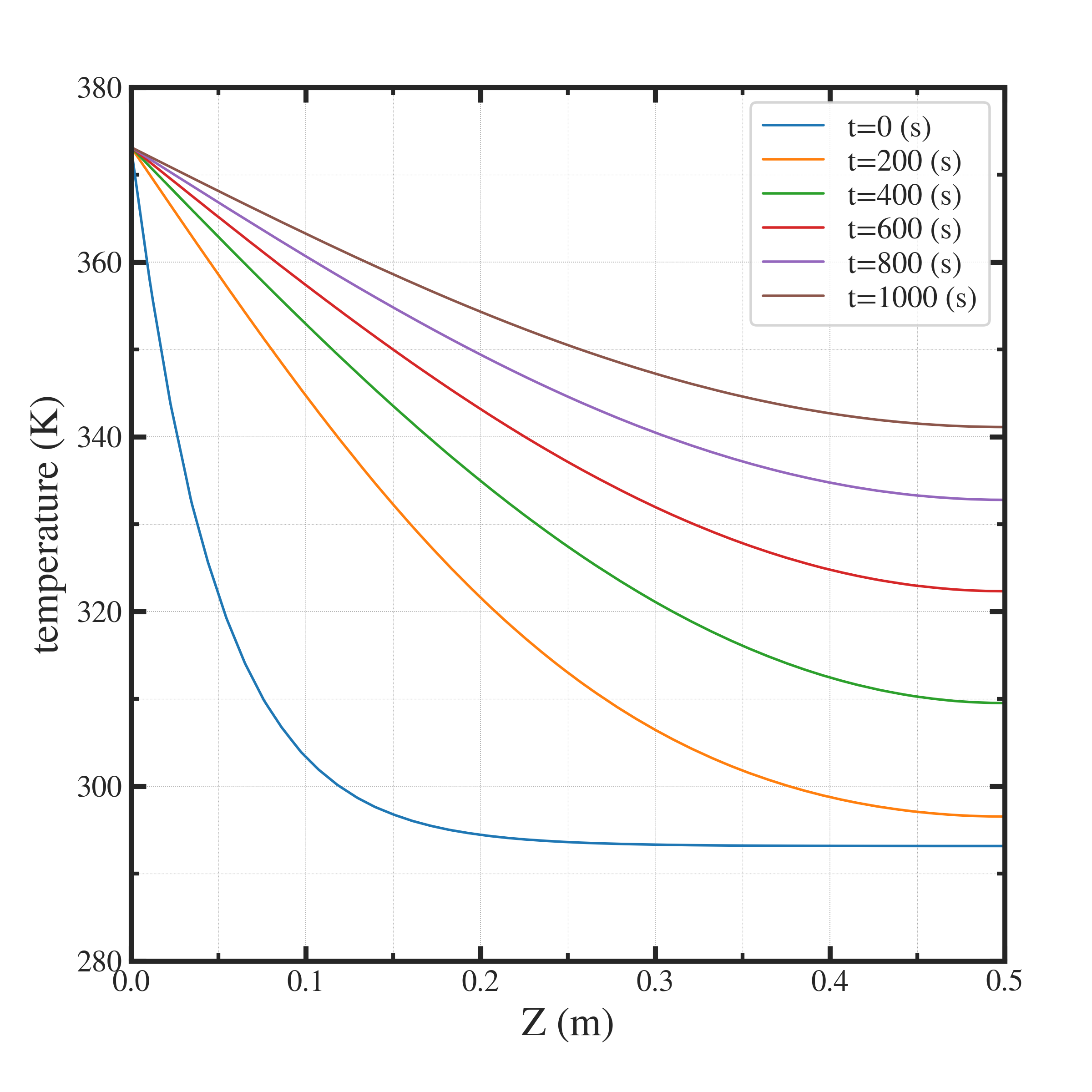
シミュレーション結果¶

結果は以下の通り．

シミュレーションの定量的妥当性¶

シミュレーションで計算した時間は 1000 [s] であり、この間に、自由境界側の一端は 47-48 [K] 程度の温度が上昇している．これが定量的に妥当かどうかを確かめておく．

物性値を以下に示す．

**シミュレーションの物性値**¶
物性値	記号	値	単位
長さ	L	0.5	m
断面積	A	0.01	m2
体積	V	0.005	m3
密度 (銅)	ρ	8960	kg/m3
熱伝導率 (銅)	λ	398	W/mK
定圧比熱 (銅)	cp	379	J/kgK

熱伝達の基本式

熱伝導のFourier則は、

$d \dot{Q} = - \lambda \nabla T \Delta A$

である．これを用いて、熱伝達量は、

$d \dot{Q} = - 398 [W/mK] \times ( 80 [K] / 0.5 [m] ) \times ( 0.1 [m] )^2 = 6.4 \times 10^2 [W/m^2]$

である． 100 ℃ のお湯に一端をつけた上記寸法の銅ロッドは、オーブントースター半分程度の熱流束を伝えてくる様子．

シミュレーション時間 1000 [s] 中に伝わる熱量 $Q=640 [W] \times 1000 [s] = 6.4 \times 10^5$ が、上昇させる銅の温度 $\Delta T$ を比熱の式より求めると、

$\Delta T &= \dfrac{ \Delta U }{ \rho V c_p } = \dfrac{ 6.4 \times 10^5 }{ 8960 \times 0.005 379 } \\ &= 37.69 [K]$

となる．温度勾配を全領域で平均としているなど、かなり大雑把な見積もりであるためか、47-48 ℃ よりも小さい値となっている．実際は、温度勾配は局所的で急峻であり、37.69 [K] よりも高い温度になることが予想される．