円環コイルと棒状鉄芯が作る磁場
円筒形の磁性体材料(鉄等)の周りに円環コイルを巻いた際の磁場分布を解析する.解析では、磁性体の磁化が非線形的に変化することを加味する.そこで、電磁場解析に用いるWhitneyAVSolverを非線形モードとし、磁性体材料に対してB-H曲線を与えている.円環コイル電流と棒状鉄芯が作る磁場の解析結果を以下に示す.
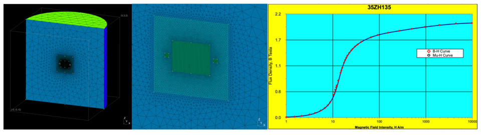
問題設定 / メッシュ
中心半径 0.65 (m) 厚さ 0.01 (m) の円環状のコイルを考え、内部を一様に直流電流 100 (kAT) が流れる.
半径 0.5 (m), 長さ 0.8 (m) の円筒形状の磁性体材料を用意する.B-H 曲線として、以下に示したデータを与える(電磁軟鉄材料)
半径 5.0 (m) 、長さ 10.0 (m) の円筒の計算空間を定義し、外周の電磁ポテンシャルに Dirichlet 条件
 を課す.
を課す.対称性は用いずにフルモデルを解く.
メッシュ生成 プログラム
gmsh-API pythonを利用した円環コイル及び棒状鉄芯のメッシュ生成プログラムを以下に示す. 自分で作成した円筒形状生成用関数を内部で利用している.
  1import numpy as np
  2import os, sys
  3import gmsh
  4
  5gmshlib = os.environ["gmshLibraryPath"]
  6sys.path.append( gmshlib )
  7
  8import generate__fanShape    as fan
  9import generate__sectorShape as sct
 10
 11# ------------------------------------------------- #
 12# --- [1] initialization of the gmsh            --- #
 13# ------------------------------------------------- #
 14gmsh.initialize()
 15gmsh.option.setNumber( "General.Terminal", 1 )
 16gmsh.model.add( "model" )
 17
 18
 19# ------------------------------------------------- #
 20# --- [2] initialize settings                   --- #
 21# ------------------------------------------------- #
 22ptsDim , lineDim , surfDim , voluDim  =  0,  1,  2,  3
 23pts    , line    , surf    , volu     = {}, {}, {}, {}
 24ptsPhys, linePhys, surfPhys, voluPhys = {}, {}, {}, {}
 25lc                                    = 10.0
 26x_, y_, z_, lc_, tag_                 = 0, 1, 2, 3, 4
 27
 28
 29# ------------------------------------------------- #
 30# --- [3] Modeling                              --- #
 31# ------------------------------------------------- #
 32
 33lc_coil        = 0.02
 34lc_bar         = 0.02
 35lc_roi         = 0.05
 36lc_sim         = 1.00
 37
 38simBoundary__r = 5.0
 39simBoundary__z = 5.0
 40roiBoundary__r = 1.0
 41roiBoundary__z = 1.0
 42
 43rCoil1         = 0.60
 44rCoil2         = 0.70
 45rBar           = 0.50
 46
 47th1            =   0.0
 48th2            = 180.0
 49zoffset1       = -0.05
 50zoffset2       = -0.40
 51hCoil          = +0.10
 52hCore          = +0.80
 53
 54
 55ret1 = fan.generate__fanShape   ( lc=lc_coil, r1=rCoil1, r2=rCoil2, th1=th1, th2=th2, \
 56                                  zoffset=zoffset1, height=+hCoil, defineVolu=True, side="+" )
 57ret2 = fan.generate__fanShape   ( lc=lc_coil, r1=rCoil1, r2=rCoil2, th1=th1, th2=th2, \
 58                                  zoffset=zoffset1, height=+hCoil, defineVolu=True, side="-" )
 59ret3 = fan.generate__fanShape   ( lc=lc_bar , r1=0.0   , r2=rBar  , th1=th1, th2=th2, \
 60                                  zoffset=zoffset2, height=+hCore, defineVolu=True, side="+" )
 61ret4 = fan.generate__fanShape   ( lc=lc_bar , r1=0.0   , r2=rBar  , th1=th1, th2=th2, \
 62                                  zoffset=zoffset2, height=+hCore, defineVolu=True, side="-" )
 63
 64ret5 = fan.generate__fanShape   ( lc=lc_roi , r1=0.0, r2=roiBoundary__r, th1=th1, th2=th2, \
 65                                  zoffset=-roiBoundary__z, height=2.0*roiBoundary__z, \
 66                                  defineVolu=True, side="+" )
 67ret6 = fan.generate__fanShape   ( lc=lc_roi , r1=0.0, r2=roiBoundary__r, th1=th1, th2=th2, \
 68                                  zoffset=-roiBoundary__z, height=2.0*roiBoundary__z, \
 69                                  defineVolu=True, side="-" )
 70ret7 = fan.generate__fanShape   ( lc=lc_sim , r1=0.0, r2=simBoundary__r, th1=th1, th2=th2, \
 71                                  zoffset=-simBoundary__z, height=2.0*simBoundary__z, \
 72                                  defineVolu=True, side="+" )
 73ret8 = fan.generate__fanShape   ( lc=lc_sim , r1=0.0, r2=simBoundary__r, th1=th1, th2=th2, \
 74                                  zoffset=-simBoundary__z, height=2.0*simBoundary__z, \
 75                                  defineVolu=True, side="-" )
 76
 77gmsh.model.occ.addPoint( 0.0, 0.0, 0.0, meshSize=lc_coil )
 78gmsh.model.occ.removeAllDuplicates()
 79
 80volu["coil1"]     = ret1["volu"]["fan"]
 81volu["coil2"]     = ret2["volu"]["fan"]
 82volu["bar1"]      = ret3["volu"]["fan"]
 83volu["bar2"]      = ret4["volu"]["fan"]
 84volu["roi_Area1"] = ret5["volu"]["fan"]
 85volu["roi_Area2"] = ret6["volu"]["fan"]
 86volu["sim_Area1"] = ret7["volu"]["fan"]
 87volu["sim_Area2"] = ret8["volu"]["fan"]
 88
 89surf["sim_top1"]  = 34
 90surf["sim_bot1"]  = 32
 91surf["sim_bot2"]  = 37
 92surf["sim_top2"]  = 39
 93surf["sim_side1"] = 33
 94surf["sim_side2"] = 36
 95surf["sim_side3"] = 38
 96surf["sim_side4"] = 40
 97
 98# ------------------------------------------------- #
 99# --- [4] Physical Grouping                     --- #
100# ------------------------------------------------- #
101gmsh.model.occ.synchronize()
102voluPhys["coil1"]     = gmsh.model.addPhysicalGroup( voluDim, [ volu["coil1"    ] ], tag=301 )
103voluPhys["coil2"]     = gmsh.model.addPhysicalGroup( voluDim, [ volu["coil2"    ] ], tag=302 )
104voluPhys["bar1"]      = gmsh.model.addPhysicalGroup( voluDim, [ volu["bar1"     ] ], tag=303 )
105voluPhys["bar2"]      = gmsh.model.addPhysicalGroup( voluDim, [ volu["bar2"     ] ], tag=304 )
106voluPhys["roi_Area1"] = gmsh.model.addPhysicalGroup( voluDim, [ volu["roi_Area1"] ], tag=305 )
107voluPhys["roi_Area2"] = gmsh.model.addPhysicalGroup( voluDim, [ volu["roi_Area2"] ], tag=306 )
108voluPhys["sim_Area1"] = gmsh.model.addPhysicalGroup( voluDim, [ volu["sim_Area1"] ], tag=307 )
109voluPhys["sim_Area2"] = gmsh.model.addPhysicalGroup( voluDim, [ volu["sim_Area2"] ], tag=308 )
110
111surfPhys["sim_bot1"]  = gmsh.model.addPhysicalGroup( surfDim, [ surf["sim_bot1" ] ], tag=201 )
112surfPhys["sim_bot2"]  = gmsh.model.addPhysicalGroup( surfDim, [ surf["sim_bot2" ] ], tag=202 )
113surfPhys["sim_top1"]  = gmsh.model.addPhysicalGroup( surfDim, [ surf["sim_top1" ] ], tag=203 )
114surfPhys["sim_top2"]  = gmsh.model.addPhysicalGroup( surfDim, [ surf["sim_top2" ] ], tag=204 )
115surfPhys["sim_side1"] = gmsh.model.addPhysicalGroup( surfDim, [ surf["sim_side1"] ], tag=205 )
116surfPhys["sim_side2"] = gmsh.model.addPhysicalGroup( surfDim, [ surf["sim_side2"] ], tag=206 )
117surfPhys["sim_side3"] = gmsh.model.addPhysicalGroup( surfDim, [ surf["sim_side3"] ], tag=207 )
118surfPhys["sim_side4"] = gmsh.model.addPhysicalGroup( surfDim, [ surf["sim_side4"] ], tag=208 )
119
120# ------------------------------------------------- #
121# --- [2] post process                          --- #
122# ------------------------------------------------- #
123gmsh.model.occ.synchronize()
124gmsh.model.mesh.generate(3)
125gmsh.write( "model.geo_unrolled" )
126gmsh.write( "model.msh" )
127gmsh.finalize()
128
Elmer入力ファイル
以下にElmer入力ファイルのサンプルを示す.
  1! ========================================================= !
  2! ===  ring and core                                    === !
  3! ========================================================= !
  4
  5! ------------------------------------------------- !
  6! --- [1] Global Simulation Settings            --- !
  7! ------------------------------------------------- !
  8
  9CHECK KEYWORDS "Warn"
 10
 11Header
 12  Mesh DB "." "model"
 13  Include Path ""
 14  Results Directory ""
 15End
 16
 17Simulation
 18  coordinate system           = "Cartesian"
 19  Coordinate Mapping(3)       = 1 2 3
 20
 21  Simulation Type             = "Steady State"
 22  Steady State Max Iterations = 1
 23
 24  Solver Input File           = "ring_and_core.sif"
 25  Output File                 = "ring_and_core.dat"
 26  Post File                   = "ring_and_core.vtu"
 27End
 28
 29
 30Constants
 31  Permeability of Vacuum = 1.2566e-06
 32End
 33
 34
 35! ------------------------------------------------- !
 36! --- [2] Body & Material Settings              --- !
 37! ------------------------------------------------- !
 38
 39Body 1
 40  Target Bodies(2) = 301 302
 41  Name             = "coil"
 42
 43  Equation         = 1
 44  Material         = 1
 45  Body Force       = 1
 46End
 47
 48Body 2
 49  Target Bodies(2) = 303 304
 50  Name             = "core"
 51
 52  Equation         = 2
 53  Material         = 2
 54End
 55
 56Body 3
 57  Target Bodies(4) = 305 306 307 308
 58  Name             = "Air"
 59
 60  Equation         = 2
 61  Material         = 3
 62End
 63
 64
 65Material 1
 66  Name                  = "Cupper"
 67  Electric Conductivity = 5.0e4
 68  Relative Permittivity = 1.0
 69  Relative Permeability = 1.0
 70End
 71
 72Material 2
 73  Name                  = "Iron"
 74  Electric Conductivity = 5.0e4
 75  Relative Permittivity = 1.0
 76  Relative Permeability = 2000.0
 77
 78  B-H Curve(38,2) = Real
 79      INCLUDE BHcurve.dat
 80End
 81
 82Material 3
 83  Name                  = "Air"
 84  Electric Conductivity = 0.0
 85  Relative Permittivity = 1.0
 86  Relative Permeability = 1.0
 87End
 88
 89
 90Component 1
 91  Name                    = "Coil"
 92  Coil Type               = "test"
 93  Master Bodies(1)        = 1
 94  Desired Coil Current    = +1.0e5
 95End
 96
 97! ------------------------------------------------- !
 98! --- [3] Equation & Solver Settings            --- !
 99! ------------------------------------------------- !
100
101Equation 1
102  Name              = "MagneticField_in_Coil"
103  Active Solvers(3) = 1 2 3
104End
105
106Equation 2
107  Name              = "MagneticField_in_Air"
108  Active Solvers(2) = 2 3
109End
110
111
112Solver 1
113  Equation                            = "CoilSolver"
114  Procedure                           = "CoilSolver" "CoilSolver"
115
116  Linear System Solver                = "Iterative"
117  Linear System Preconditioning       = "ILU1"
118  Linear System Max Iterations        = 1000
119  Linear System Convergence Tolerance = 1e-08
120  Linear System Iterative Method      = "BiCGStabL"
121  Linear System Residual Output       = 20
122  Steady State Convergence Tolerance  = 1e-06
123
124  Optimize Bandwidth                  = True
125  Nonlinear System Consistent Norm    = True
126  Coil Closed                         = Logical True
127  Narrow Interface                    = Logical False
128
129  Normalize Coil Current              = Logical True
130  Save Coil Set                       = Logical False
131  Save Coil Index                     = Logical False
132  Calculate Elemental Fields          = Logical True
133End
134
135Solver 2
136  Equation                            = "WhitneySolver"
137  Variable                            = "AV"
138  Variable Dofs                       = 1
139  Procedure                           = "MagnetoDynamics" "WhitneyAVSolver"
140
141  Linear System Solver                = "Iterative"
142  Linear System Iterative Method      = "BiCGStab"
143  Linear System Max Iterations        = 3000
144  Linear System Convergence Tolerance = 1.0e-4
145  Linear System Preconditioning       = "None"
146  Linear System Symmetric             = True
147
148  Steady State Convergence Tolerance       = 1.0e-5
149  Nonlinear System Convergence Tolerance   = 1.0e-8
150  Nonlinear System Max Iterations          = 3
151  Nonlinear System Newton After Iterations = 3
152  Nonlinear System Newton After Tolerance  = 1.0e-8
153  Nonlinear System Relaxation Factor       = 0.5
154End
155
156Solver 3
157  Equation                            = "MGDynamicsCalc"
158  Procedure                           = "MagnetoDynamics" "MagnetoDynamicsCalcFields"
159  Potential Variable                  = String "AV"
160
161  Calculate Current Density           = Logical True
162  Calculate Magnetic Field Strength   = Logical True
163
164  Steady State Convergence Tolerance  = 0
165  Linear System Solver                = "Iterative"
166  Linear System Preconditioning       = None
167  Linear System Residual Output       = 0
168  Linear System Max Iterations        = 5000
169  Linear System Iterative Method      = "CG"
170  Linear System Convergence Tolerance = 1.0e-8
171  Linear System Symmetric             = True
172
173  Nonlinear System Consistent Norm    = Logical True
174  Discontinuous Bodies                = True
175End
176
177
178! ------------------------------------------------- !
179! --- [4] Body Forces / Initial Conditions      --- !
180! ------------------------------------------------- !
181
182Body Force 1
183  Name              = "CoilCurrentSource"
184  Current Density 1 = Equals "CoilCurrent e 1"
185  Current Density 2 = Equals "CoilCurrent e 2"
186  Current Density 3 = Equals "CoilCurrent e 3"
187End
188
189
190! ------------------------------------------------- !
191! --- [5] Boundary Conditions                   --- !
192! ------------------------------------------------- !
193
194Boundary Condition 1
195  Name = "Far Boundary"
196  Target Boundaries(8) = 201 202 203 204 205 206 207 208
197  AV {e}               = 0.0
198End
入力ファイルの要点は以下である.
磁場計算には WhitneyAVSolver を非線形解析で用いる.非線形計算用に、 NonLinear System Max Iterations > 1 として設定する.
Material Section にて、B-H Curve を与える.同ディレクトリにおいている BHcurve.dat を INCLUDE文で読み込み、B-H曲線を与える.
コイル電流は CoilSolver を使用して計算する.フルモデル用にループ電流を定義する( Coil Closed = True ). 付随する Component 及び、 Body Force を定義しておく. Desired Coil Current として、1.0e5 を与える.
境界条件を 辺要素 に対する指定とし( {e} を付記して指定 e:edge )、 Dirichlet 条件を課す.
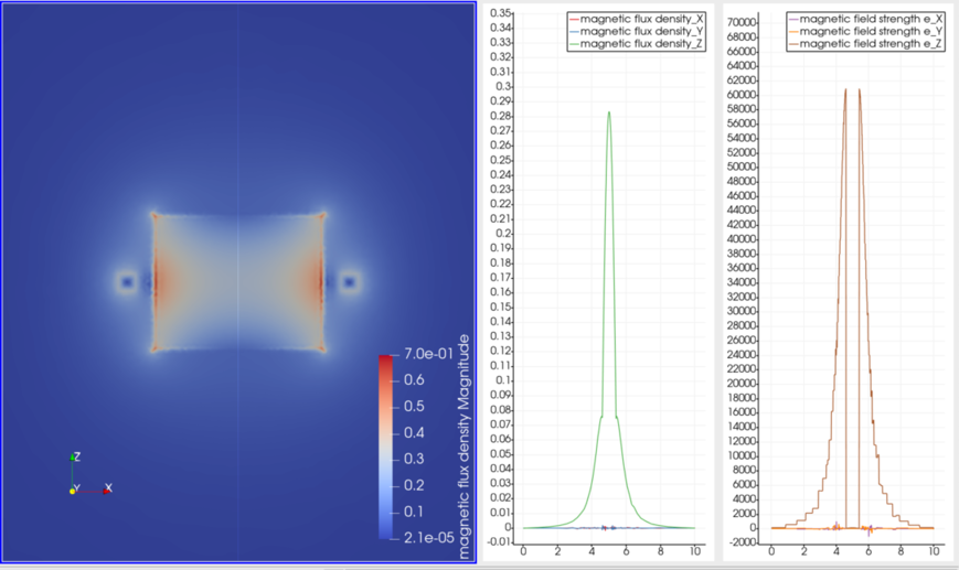
非線形磁場解析の結果
解析実行結果は以下に示す.以下にxz平面での磁束密度分布とz軸上の磁界 H 及び 磁束密度 B を示す.
xz平面での磁束密度、及び、 磁力線の3次元分布を示す.
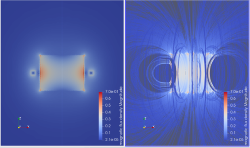
磁力線はparaviewの Stream Line を用いて描画している.