C型電磁石がつくる磁場
C型電磁石が作る磁場の解析結果を以下に示す.
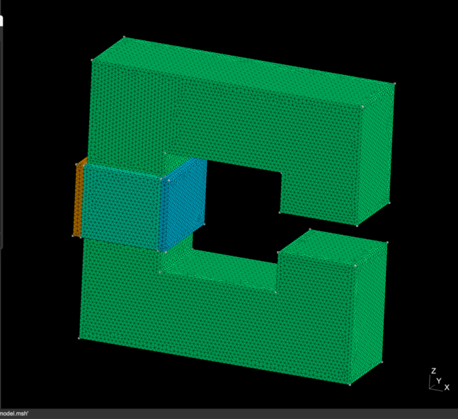
問題設定 / メッシュ
C型の鉄芯を考える.鉄芯の断面は長さ 0.2 (m) の正方形とし、鉄芯の中心経路は一辺 0.5 (m) とする(つまり、C型電磁石の一辺の合計長さは 0.1+0.5+0.1 = 0.7 (m) となる).
中心経路をつくる正方形のうち、ギャップと反対側の辺にコイルを設置する.コイルはコーナー部を除いた鉄芯直線部分のうち、60 (%) の領域に巻きつける.直線部分は長さ 0.5-0.1-0.1 = 0.3 であるからコイルの巻きつけ長さは 0.3*0.6 = 0.18 であり、コイル幅は 0.02 (m) と設定する.コイル電流は 100 kA とする.
計算領域は、1辺 2.0 (m) の立方体の計算空間を考え、境界で電磁ポテンシャルは Dirichlet 条件
 を課す.
を課す.
C型電磁石のメッシュ生成 プログラム
メッシュ生成用プログラムを以下に示す.
  1import numpy as np
  2import os, sys
  3import gmsh_api.gmsh as gmsh
  4
  5import nkGmshRoutines.generate__quadShape  as qua
  6import nkGmshRoutines.generate__squareTube as tub
  7
  8
  9# ------------------------------------------------- #
 10# --- [1] initialization of the gmsh            --- #
 11# ------------------------------------------------- #
 12gmsh.initialize()
 13gmsh.option.setNumber( "General.Terminal", 1 )
 14gmsh.model.add( "model" )
 15
 16# ------------------------------------------------- #
 17# --- [2] initialize settings                   --- #
 18# ------------------------------------------------- #
 19ptsDim , lineDim , surfDim , voluDim  =  0,  1,  2,  3
 20pts    , line    , surf    , volu     = {}, {}, {}, {}
 21ptsPhys, linePhys, surfPhys, voluPhys = {}, {}, {}, {}
 22x_, y_, z_, lc_, tag_                 =  0,  1,  2,  3, 4
 23
 24# ------------------------------------------------- #
 25# --- [3] Modeling                              --- #
 26# ------------------------------------------------- #
 27
 28lc_sim     =  0.800
 29lc_mag     =  0.010
 30lc_coil    =  0.010
 31
 32gap        =  0.100
 33Lmag       =  0.500
 34Lsquare    =  0.200
 35coil_width =  0.020
 36
 37# ------------------------------------------------- #
 38# --- C-shaped Magnet core                      --- #
 39# ------------------------------------------------- #
 40
 41Ledge_out  =   0.5*Lmag + 0.5*Lsquare
 42Ledge_inn  =   0.5*Lmag - 0.5*Lsquare
 43Lhalf_gap  =   0.5*gap
 44y_minus    = - 0.5*Lsquare
 45
 46pts["x1" ] = [ -Ledge_out, y_minus, -Ledge_out, lc_mag, 0 ]
 47pts["x2" ] = [ +Ledge_out, y_minus, -Ledge_out, lc_mag, 0 ]
 48pts["x3" ] = [ +Ledge_out, y_minus, -Lhalf_gap, lc_mag, 0 ]
 49pts["x4" ] = [ +Ledge_inn, y_minus, -Lhalf_gap, lc_mag, 0 ]
 50pts["x5" ] = [ +Ledge_inn, y_minus, -Ledge_inn, lc_mag, 0 ]
 51pts["x6" ] = [ -Ledge_inn, y_minus, -Ledge_inn, lc_mag, 0 ]
 52pts["x7" ] = [ -Ledge_inn, y_minus, +Ledge_inn, lc_mag, 0 ]
 53pts["x8" ] = [ +Ledge_inn, y_minus, +Ledge_inn, lc_mag, 0 ]
 54pts["x9" ] = [ +Ledge_inn, y_minus, +Lhalf_gap, lc_mag, 0 ]
 55pts["x10"] = [ +Ledge_out, y_minus, +Lhalf_gap, lc_mag, 0 ]
 56pts["x11"] = [ +Ledge_out, y_minus, +Ledge_out, lc_mag, 0 ]
 57pts["x12"] = [ -Ledge_out, y_minus, +Ledge_out, lc_mag, 0 ]
 58
 59# -- add points -- #
 60for key in list( pts.keys() ):
 61    pts[key][4] = gmsh.model.occ.addPoint( pts[key][0], pts[key][1], pts[key][2], meshSize=pts[key][3] )
 62
 63# -- add lines  -- #
 64lineLoop = []
 65index    = [ ik+1 for ik in range(12) ] + [1]
 66for ik in range( len( index )-1 ):
 67    ik1, ik2       = index[ik], index[ik+1]
 68    ptkey1, ptkey2 = "x{0}".format(ik1), "x{0}".format(ik2)
 69    linekey        = "line_{0}_{1}".format(ik1,ik2)
 70    line[linekey]  = gmsh.model.occ.addLine( pts[ptkey1][tag_], pts[ptkey2][tag_] )
 71    lineLoop.append( line[linekey] )
 72
 73# -- add surface  -- #
 74lineGroup          = gmsh.model.occ.addCurveLoop( lineLoop )
 75surf["cMag"]       = gmsh.model.occ.addPlaneSurface( [ lineGroup ] )
 76
 77# -- add volume   -- #
 78delta              = [ 0.0, Lsquare, 0.0 ]
 79ret1               = gmsh.model.occ.extrude( [ (surfDim,surf["cMag"]) ], delta[0], delta[1], delta[2] )
 80volu["cMag"]       = ret1[1][1]
 81
 82
 83# ------------------------------------------------- #
 84# --- coil around magnetic core                 --- #
 85# ------------------------------------------------- #
 86
 87coil_length  = ( Lmag - Lsquare ) * 0.6
 88xcent        = - 0.5*Lmag
 89ycent        =   0.0
 90d_in         =   0.5*Lsquare
 91d_out        =   0.5*Lsquare + coil_width
 92z_bot        = - 0.5*coil_length
 93z_top        = + 0.5*coil_length
 94
 95vL1_coil_1   = [ xcent-d_out, ycent-d_out, z_bot ]
 96vL1_coil_2   = [ xcent-d_in , ycent-d_out, z_bot ]
 97vL1_coil_3   = [ xcent-d_in , ycent-d_out, z_top ]
 98vL1_coil_4   = [ xcent-d_out, ycent-d_out, z_top ]
 99delta1       = [         0.0,   2.0*d_out,   0.0 ]
100
101vL2_coil_1   = [ xcent-d_in , ycent-d_out, z_bot ]
102vL2_coil_2   = [ xcent+d_in , ycent-d_out, z_bot ]
103vL2_coil_3   = [ xcent+d_in , ycent-d_out, z_top ]
104vL2_coil_4   = [ xcent-d_in , ycent-d_out, z_top ]
105delta2       = [         0.0,  coil_width,   0.0 ]
106
107vL3_coil_1   = [ xcent-d_in , ycent+d_in , z_bot ]
108vL3_coil_2   = [ xcent+d_in , ycent+d_in , z_bot ]
109vL3_coil_3   = [ xcent+d_in , ycent+d_in , z_top ]
110vL3_coil_4   = [ xcent-d_in , ycent+d_in , z_top ]
111delta3       = [         0.0,  coil_width,   0.0 ]
112
113vL4_coil_1   = [ xcent+d_in , ycent-d_out, z_bot ]
114vL4_coil_2   = [ xcent+d_out, ycent-d_out, z_bot ]
115vL4_coil_3   = [ xcent+d_out, ycent-d_out, z_top ]
116vL4_coil_4   = [ xcent+d_in , ycent-d_out, z_top ]
117delta4       = [         0.0,   2.0*d_out,   0.0 ]
118
119ret2_1       = qua.generate__quadShape( lc=lc_coil, extrude_delta=delta1, defineVolu=True, \
120                                        x1=vL1_coil_1, x2=vL1_coil_2, \
121                                        x3=vL1_coil_3, x4=vL1_coil_4  )
122ret2_2       = qua.generate__quadShape( lc=lc_coil, extrude_delta=delta2, defineVolu=True, \
123                                        x1=vL2_coil_1, x2=vL2_coil_2, \
124                                        x3=vL2_coil_3, x4=vL2_coil_4  )
125ret2_3       = qua.generate__quadShape( lc=lc_coil, extrude_delta=delta3, defineVolu=True, \
126                                        x1=vL3_coil_1, x2=vL3_coil_2, \
127                                        x3=vL3_coil_3, x4=vL3_coil_4  )
128ret2_4       = qua.generate__quadShape( lc=lc_coil, extrude_delta=delta4, defineVolu=True, \
129                                        x1=vL4_coil_1, x2=vL4_coil_2, \
130                                        x3=vL4_coil_3, x4=vL4_coil_4  )
131volu["coil1"] = ret2_1["volu"]["quad"]
132volu["coil2"] = ret2_2["volu"]["quad"]
133volu["coil3"] = ret2_3["volu"]["quad"]
134volu["coil4"] = ret2_4["volu"]["quad"]
135
136# ------------------------------------------------- #
137# --- simulation region                         --- #
138# ------------------------------------------------- #
139
140simulation_region = "box"
141
142if ( simulation_region == "box" ):
143    xSim    = 2.0
144    ySim    = 2.0
145    zSim    = 2.0
146
147    x1_sim  = [ -xSim, -ySim,    -zSim ]
148    x2_sim  = [ -xSim, +ySim,    -zSim ]
149    x3_sim  = [ +xSim, +ySim,    -zSim ]
150    x4_sim  = [ +xSim, -ySim,    -zSim ]
151    delta   = [   0.0,   0.0, 2.0*zSim ]
152    ret3    = qua.generate__quadShape( lc=lc_sim, x1=x1_sim, x2=x2_sim, x3=x3_sim, x4=x4_sim, \
153                                       extrude_delta=delta, defineVolu=True )
154    volu["air"] = ret3["volu"]["quad"]
155
156elif ( simulation_region == "sphere" ):
157    sph     = [ 0.0, 0.0, 0.0, 2.0 ]
158    ret     = gmsh.model.occ.addSphere( sph[0], sph[1], sph[2], sph[3] )
159    volu["air"] = ret
160
161
162# ------------------------------------------------- #
163# --- [4] Physical Grouping                     --- #
164# ------------------------------------------------- #
165
166gmsh.model.occ.removeAllDuplicates()
167
168farBCs  = [ 28, 29, 30, 31, 32, 33 ]
169
170gmsh.model.occ.synchronize()
171voluPhys["cMag"] = gmsh.model.addPhysicalGroup( voluDim, [ volu["cMag"] ], tag=301 )
172voluPhys["coil"] = gmsh.model.addPhysicalGroup( voluDim, [ volu["coil1"], volu["coil2"], \
173                                                           volu["coil3"], volu["coil4"] ], tag=302 )
174voluPhys["air"]  = gmsh.model.addPhysicalGroup( voluDim, [ volu["air"]  ], tag=303 )
175
176surfPhys["far"]  = gmsh.model.addPhysicalGroup( surfDim, farBCs, tag=201 )
177
178# ------------------------------------------------- #
179# --- [2] post process                          --- #
180# ------------------------------------------------- #
181gmsh.model.occ.synchronize()
182gmsh.model.mesh.generate(3)
183gmsh.write( "model.geo_unrolled" )
184gmsh.write( "model.msh" )
185gmsh.finalize()
186
C型電磁石の磁場解析用 Elmer入力ファイル
以下にElmer入力ファイルのサンプルを示す.
  1! ========================================================= !
  2! ===  C-Shape Magnet and coil                          === !
  3! ========================================================= !
  4
  5! ------------------------------------------------- !
  6! --- [1] Global Simulation Settings            --- !
  7! ------------------------------------------------- !
  8
  9CHECK KEYWORDS "Warn"
 10
 11Header
 12  Mesh DB "." "model"
 13  Include Path ""
 14  Results Directory ""
 15End
 16
 17Simulation
 18  coordinate system           = "Cartesian"
 19  Coordinate Mapping(3)       = 1 2 3
 20
 21  Simulation Type             = "Steady State"
 22  Steady State Max Iterations = 1
 23
 24  Solver Input File           = "cShape_magnet.sif"
 25  Output File                 = "cShape_magnet.dat"
 26  Post File                   = "cShape_magnet.vtu"
 27End
 28
 29
 30Constants
 31  Permeability of Vacuum = 1.2566e-06
 32End
 33
 34
 35! ------------------------------------------------- !
 36! --- [2] Body & Material Settings              --- !
 37! ------------------------------------------------- !
 38
 39Body 1
 40  Target Bodies(1) = 302
 41  Name             = "coil"
 42
 43  Equation         = 1
 44  Material         = 1
 45  Body Force       = 1
 46End
 47
 48Body 2
 49  Target Bodies(1) = 301
 50  Name             = "core"
 51
 52  Equation         = 2
 53  Material         = 2
 54End
 55
 56Body 3
 57  Target Bodies(1) = 303
 58  Name             = "air"
 59
 60  Equation         = 2
 61  Material         = 3
 62End
 63
 64
 65Material 1
 66  Name                  = "Cupper"
 67  Electric Conductivity = 5.0e7
 68  Relative Permittivity = 1.0
 69  Relative Permeability = 1.0
 70End
 71
 72Material 2
 73  Name                  = "Iron"
 74  Electric Conductivity = 1.0e7
 75  Relative Permittivity = 1.0
 76  Relative Permeability = 5000
 77
 78  H-B Curve(38,2) = Real
 79      INCLUDE HBcurve.dat
 80End
 81
 82Material 3
 83  Name                  = "Air"
 84  Electric Conductivity = 0.0
 85  Relative Permittivity = 1.0
 86  Relative Permeability = 1.0
 87End
 88
 89
 90Component 1
 91  Name                    = "Coil"
 92  Coil Type               = "test"
 93  Master Bodies(1)        = 1
 94  Desired Coil Current    = +1.0e5
 95End
 96
 97! ------------------------------------------------- !
 98! --- [3] Equation & Solver Settings            --- !
 99! ------------------------------------------------- !
100
101Equation 1
102  Name              = "MagneticField_in_Coil"
103  Active Solvers(3) = 1 2 3
104End
105
106Equation 2
107  Name              = "MagneticField_in_Material"
108  Active Solvers(2) = 2 3
109End
110
111
112Solver 1
113  Equation                            = "CoilSolver"
114  Procedure                           = "CoilSolver" "CoilSolver"
115
116  Linear System Solver                = "Iterative"
117  Linear System Preconditioning       = "ILU1"
118  Linear System Max Iterations        = 3000
119  Linear System Convergence Tolerance = 1e-08
120  Linear System Iterative Method      = "BiCGStabL"
121  Linear System Residual Output       = 20
122  Steady State Convergence Tolerance  = 1e-06
123
124  Optimize Bandwidth                  = True
125  Nonlinear System Consistent Norm    = True
126  Coil Closed                         = Logical True
127  Narrow Interface                    = Logical False
128
129  Normalize Coil Current              = Logical True
130  Save Coil Set                       = Logical False
131  Save Coil Index                     = Logical False
132  Calculate Elemental Fields          = Logical True
133End
134
135Solver 2
136  Equation                            = "WhitneySolver"
137  Variable                            = "AV"
138  Variable Dofs                       = 1
139  Procedure                           = "MagnetoDynamics" "WhitneyAVSolver"
140
141  Linear System Solver                = "Iterative"
142  Linear System Iterative Method      = "BiCGStab"
143  Linear System Max Iterations        = 3000
144  Linear System Convergence Tolerance = 1.0e-6
145  Linear System Preconditioning       = "None"
146  Linear System Symmetric             = True
147
148  Steady State Convergence Tolerance       = 1.0e-6
149  Nonlinear System Convergence Tolerance   = 1.0e-8
150  Nonlinear System Max Iterations          = 100
151  Nonlinear System Newton After Iterations = 3
152  Nonlinear System Newton After Tolerance  = 1.0e-8
153  Nonlinear System Relaxation Factor       = 0.5
154End
155
156Solver 3
157  Equation                            = "MGDynamicsCalc"
158  Procedure                           = "MagnetoDynamics" "MagnetoDynamicsCalcFields"
159  Potential Variable                  = String "AV"
160
161  Calculate Current Density           = Logical True
162  Calculate Magnetic Field Strength   = Logical True
163
164  Steady State Convergence Tolerance  = 0
165  Linear System Solver                = "Iterative"
166  Linear System Preconditioning       = None
167  Linear System Residual Output       = 0
168  Linear System Max Iterations        = 5000
169  Linear System Iterative Method      = "CG"
170  Linear System Convergence Tolerance = 1.0e-8
171  Linear System Symmetric             = True
172
173  Nonlinear System Consistent Norm    = Logical True
174  Discontinuous Bodies                = True
175End
176
177
178! ------------------------------------------------- !
179! --- [4] Body Forces / Initial Conditions      --- !
180! ------------------------------------------------- !
181
182Body Force 1
183  Name              = "CoilCurrentSource"
184  Current Density 1 = Equals "CoilCurrent e 1"
185  Current Density 2 = Equals "CoilCurrent e 2"
186  Current Density 3 = Equals "CoilCurrent e 3"
187End
188
189
190! ------------------------------------------------- !
191! --- [5] Boundary Conditions                   --- !
192! ------------------------------------------------- !
193
194Boundary Condition 1
195  Name = "Far Boundary"
196  Target Boundaries(1) = 201
197  AV {e}               = 0.0
198End
C型電磁石の入力ファイルの要点は以下である.
H-B Curveにより H-B 曲線をデータとして与えている.
Body 1 に付随する component を定義し、無次元量として理想電流 100 (kA) を与えている.
Body Force を定義し、componentが作っている電流を体積力として定義している.
Coil Closed を True としている.
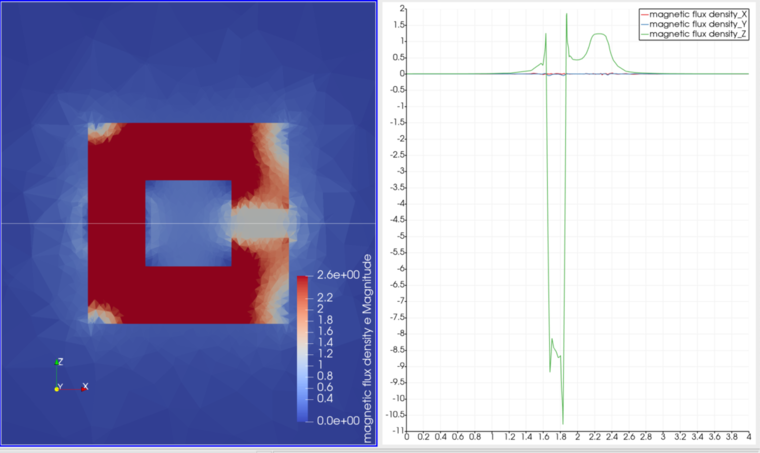
円環コイル電流がつくる磁場の解析結果
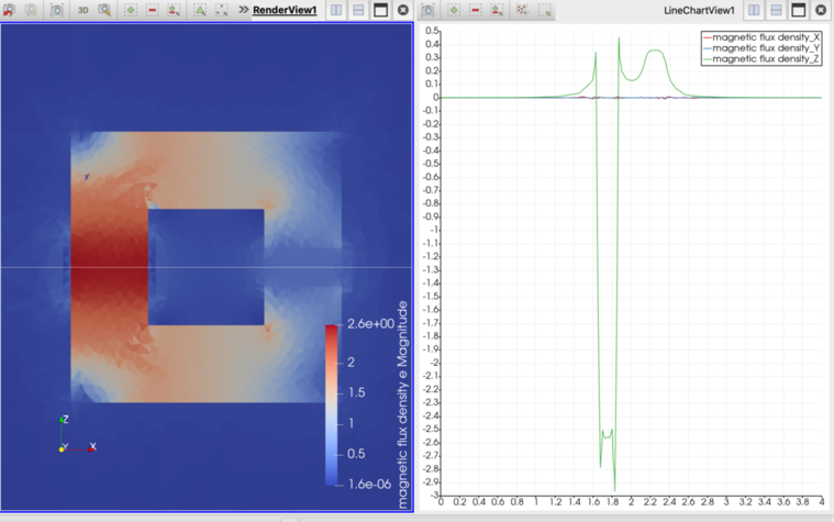
解析実行結果は以下に示す.以下に電流密度分布と軸方向の磁束密度を示す.
C型電磁石 がギャップ間につくる磁場は、アンペールの法則より、
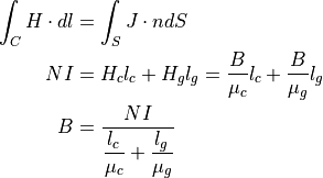
もし、C型電磁石のように鉄芯の透磁率が真空の透磁率に比べて十分大きい場合( 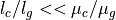 )、磁場は、

と計算できる.これは、磁気回路において、導線に相当する鉄芯において起磁力降下が生じないことを意味している.つまり、全ての起磁力はギャップ間での磁場の発生のために使われていることになる.上式を用いて、ギャップ間の磁場を計算すると、
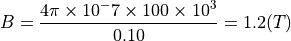
である.
一方、FEMにより磁場解析の結果ではギャップ近辺での磁場は 0.36 (T) であり、1/4程度となっている. これは、定義した H-B 曲線による比透磁率が 100 程度であるため、磁気抵抗が大きく、有限の起磁力降下が鉄芯内で生じたことにより、磁場が小さくなっていると考えられる.
参考例として、以下に、H-B 曲線をコメントアウトし、非透磁率 5000 一定で線形計算した場合の磁場分布を示す.
こちらでは、上記の過程が概ね成立し、ギャップ間において、1.2 (T) 磁場強度が得られている.