H型電磁石がつくる磁場
H型電磁石が作る磁場の解析結果を以下に示す.
問題設定 / メッシュ
座標系として軸対称の円筒座標系を考える.計算平面は x-z座標とする.
H型の鉄芯を考える.磁極半径は 0.670 (m) とし、鉄芯の各部寸法は適宜与えるものとする.
H型鉄芯のコイルスロット部にコイルを設定する.コイル電流としては、1.76 (MAT) を与えるものとする.
計算領域は、磁極モデルに加えて厚さ 2.0 (m) の空気層を追加した領域を対象とする.
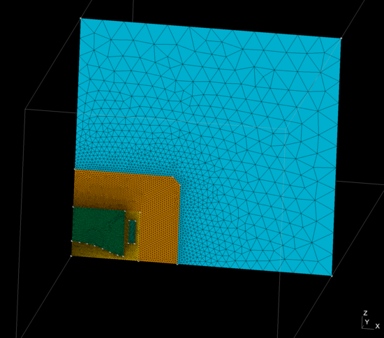
H型電磁石のメッシュ生成 プログラム
メッシュ生成用プログラムを以下に示す.
  1import os, sys
  2import numpy                       as np
  3import gmsh_api.gmsh               as gmsh
  4import nkUtilities.load__constants as lcn
  5import nkGmshRoutines.generate__polygon as ply
  6
  7# ------------------------------------------------- #
  8# --- [1] initialization of the gmsh            --- #
  9# ------------------------------------------------- #
 10gmsh.initialize()
 11gmsh.option.setNumber( "General.Terminal", 1 )
 12gmsh.option.setNumber( "Mesh.Algorithm"  , 6 )
 13gmsh.option.setNumber( "Mesh.Algorithm3D", 1 )
 14gmsh.model.add( "model" )
 15
 16# ------------------------------------------------- #
 17# --- [2] initialize settings                   --- #
 18# ------------------------------------------------- #
 19ptsDim , lineDim , surfDim , voluDim  =  0,  1,  2,  3
 20pts    , line    , surf    , volu     = {}, {}, {}, {}
 21ptsPhys, linePhys, surfPhys, voluPhys = {}, {}, {}, {}
 22x_, y_, z_, lc_, tag_                 =  0,  1,  2,  3, 4
 23
 24
 25# ------------------------------------------------- #
 26# --- [3] Parameter Settings                    --- #
 27# ------------------------------------------------- #
 28
 29tolerance       = 1.e-5
 30const           = lcn.load__constants( inpFile   ="dat/magnet.conf" )
 31mesh_conf       = lcn.load__constants( inpFile   ="dat/mesh.conf"   )
 32
 33lc1             = mesh_conf["volu1_mesh"]
 34lc4             = mesh_conf["volu4_mesh"]
 35lc5             = mesh_conf["volu5_mesh"]
 36lc6             = mesh_conf["volu6_mesh"]
 37lc7             = mesh_conf["volu7_mesh"]
 38lc8             = mesh_conf["volu8_mesh"]
 39
 40z_slotDepth     = const["z_medianPlane"] + const["z_airGap1"] + const["z_coilWidth"] + const["z_airGap2"]
 41
 42rPole1          = const["r_poleRadius"]
 43zPole1          = const["z_medianPlane"]
 44zPole3          = const["z_poleGapMax"]
 45zPole4          = z_slotDepth
 46
 47rBuff1          = const["r_poleRadius"]
 48rBuff2          = const["r_poleRadius"]  + const["r_airGap1"]
 49zBuff1          = const["z_medianPlane"]
 50zBuff2          = z_slotDepth
 51
 52rCoil1          = const["r_poleRadius"]  + const["r_airGap1"]
 53rCoil2          = const["r_poleRadius"]  + const["r_airGap1"] + const["r_coilWidth"]
 54rCoil3          = const["r_poleRadius"]  + const["r_airGap1"] + const["r_coilWidth"] + const["r_airGap2"]
 55zCoil1          = const["z_medianPlane"]
 56zCoil2          = const["z_medianPlane"] + const["z_airGap1"]
 57zCoil3          = const["z_medianPlane"] + const["z_airGap1"] + const["z_coilWidth"]
 58zCoil4          = const["z_medianPlane"] + const["z_airGap1"] + const["z_coilWidth"] + const["z_airGap2"]
 59
 60rYoke1          = const["r_poleRadius"]  + const["r_airGap1"] + const["r_coilWidth"] + const["r_airGap2"]
 61rYoke2          = rYoke1 + const["r_yokeWidth"] - const["r_yokeCorner"]
 62rYoke3          = rYoke1 + const["r_yokeWidth"]
 63zYoke1          = const["z_medianPlane"]
 64zYoke2          = z_slotDepth
 65zYoke3          = z_slotDepth + const["z_yokeWidth"] - const["z_yokeCorner"]
 66zYoke4          = z_slotDepth + const["z_yokeWidth"]
 67
 68rAir1           = rYoke1 + const["r_yokeWidth"] - const["r_yokeCorner"]
 69rAir2           = rYoke1 + const["r_yokeWidth"]
 70rAir3           = rYoke1 + const["r_yokeWidth"] + const["r_outAirWidth"]
 71zAir1           = const["z_medianPlane"]
 72zAir2           = z_slotDepth + const["z_yokeWidth"] - const["z_yokeCorner"]
 73zAir3           = z_slotDepth + const["z_yokeWidth"]
 74zAir4           = z_slotDepth + const["z_yokeWidth"] + const["z_outAirWidth"]
 75
 76zRegen          = const["z_regenCeil"]
 77zPeeler         = const["z_peelerBottom"]
 78
 79
 80# ------------------------------------------------- #
 81# --- [4] Modeling pole                         --- #
 82# ------------------------------------------------- #
 83
 84inpFile = "dat/pole_cs.dat"
 85with open( inpFile, "r" ) as f:
 86    rData   = np.loadtxt( f )
 87
 88pole_vertex        = np.zeros( (rData.shape[0]+2,3) )
 89pole_vertex[:-2,:] =   rData
 90pole_vertex[ -2,:] = [ rPole1, 0.0, zYoke2 ]
 91pole_vertex[ -1,:] = [    0.0, 0.0, zYoke2 ]
 92
 93ret1 = ply.generate__polygon( lc=lc1, vertex=pole_vertex )
 94
 95
 96# ------------------------------------------------- #
 97# --- [5] Modeling yoke                         --- #
 98# ------------------------------------------------- #
 99
100xY1         = [    0.0, 0.0, zYoke2 ]
101xY2         = [ rPole1, 0.0, zYoke2 ]
102xY3         = [ rYoke1, 0.0, zYoke2 ]
103xY4         = [ rYoke1, 0.0, zYoke1 ]
104xY5         = [ rYoke3, 0.0, zYoke1 ]
105xY6         = [ rYoke3, 0.0, zYoke3 ]
106xY7         = [ rYoke2, 0.0, zYoke4 ]
107xY8         = [    0.0, 0.0, zYoke4 ]
108yoke_vertex = np.array( [ xY1, xY2, xY3, xY4, xY5, xY6, xY7, xY8 ] )
109
110ret2        = ply.generate__polygon( lc=lc6, vertex=yoke_vertex )
111
112
113# ------------------------------------------------- #
114# --- [6] coil Modeling                         --- #
115# ------------------------------------------------- #
116
117xc1         = [ rCoil1, 0.0, zCoil2 ]
118xc2         = [ rCoil2, 0.0, zCoil2 ]
119xc3         = [ rCoil2, 0.0, zCoil3 ]
120xc4         = [ rCoil1, 0.0, zCoil3 ]
121coil_vertex = np.array( [ xc1, xc2, xc3, xc4 ] )
122
123ret3        = ply.generate__polygon( lc=lc5, vertex=coil_vertex )
124
125
126# ------------------------------------------------- #
127# --- [7] simulation region                     --- #
128# ------------------------------------------------- #
129
130xS1         = [   0.0, 0.0,   0.0, lc1, 0 ] # lc1 should be used
131xS2         = [ rAir3, 0.0,   0.0, lc7, 0 ]
132xS3         = [ rAir3, 0.0, zAir4, lc7, 0 ]
133xS4         = [   0.0, 0.0, zAir4, lc7, 0 ]
134simu_vertex = np.array( [ xS1, xS2, xS3, xS4 ] )
135
136ret4        = ply.generate__polygon( lc=lc7, vertex=simu_vertex )
137
138
139# ------------------------------------------------- #
140# --- [8] remove Duplicates / physNum Grouping  --- #
141# ------------------------------------------------- #
142#  -- [8-1] remove Duplicates                   --  #
143gmsh.model.occ.removeAllDuplicates()
144
145#  -- [8-2] physical Grouping                   --  #
146
147pntFile = "dat/physNumTable.conf"
148import nkGmshRoutines.load__physNumTable as pnt
149ret     = pnt.load__physNumTable( inpFile =pntFile , line    =line    , surf    =surf, volu=volu, \
150                                  linePhys=linePhys, surfPhys=surfPhys, voluPhys=voluPhys )
151
152# ------------------------------------------------- #
153# --- [9] post process                          --- #
154# ------------------------------------------------- #
155gmsh.model.occ.synchronize()
156gmsh.model.mesh.generate(2)
157# gmsh.option.setNumber( "Mesh.BdfFieldFormat", 0 )
158# gmsh.option.setNumber( "Mesh.SaveElementTagType", 2 )
159# gmsh.write( "msh/model.bdf" )
160gmsh.write( "msh/model.geo_unrolled" )
161gmsh.write( "msh/model.msh" )
162gmsh.finalize()
163
164
165
166
167
168# Data        = np.zeros( (nData,5) )
169# Data[:,0:3] = rData
170# Data[:,  3] = lc1
171# Data[:,  4] = 0
172
173# polekeys = []
174# for ik in range( nData ):
175#     key            = "pole_{0:06}".format( ik )
176#     pts[key]       = [ Data[ik,x_], Data[ik,y_], Data[ik,z_], Data[ik,lc_], Data[ik,tag_] ]
177#     pts[key][tag_] = gmsh.model.occ.addPoint( pts[key][x_], pts[key][y_], pts[key][z_], \
178#                                               meshSize=pts[key][lc_] )
179#     polekeys.append( key )
180# pts["poleRoot1"] = [ Data[ 0,x_], Data[ 0,y_], zYoke2, lc1, 0 ]
181# pts["poleRoot2"] = [ Data[-1,x_], Data[-1,y_], zYoke2, lc1, 0 ]
182# for key in ["poleRoot2","poleRoot1"]:
183#     pts[key][tag_] = gmsh.model.occ.addPoint( pts[key][x_], pts[key][y_], pts[key][z_], \
184#                                               meshSize=pts[key][lc_] )
185#     polekeys.append( key )
186
187# lineLoop = []
188# keys_1   = np.roll( np.array( polekeys ),  0 )
189# keys_2   = np.roll( np.array( polekeys ), -1 )
190# for ik in range( keys_1.shape[0] ):
191#     linekey        = "line_{0}".format( ik )
192#     line[linekey]  = gmsh.model.occ.addLine( pts[keys_1[ik]][tag_], pts[keys_2[ik]][tag_] )
193#     lineLoop.append( line[linekey] )
194
195# #  -- [2-3] generate surfaces                   --  #
196# lineGroup          = gmsh.model.occ.addCurveLoop( lineLoop )
197# surf["quad"]       = gmsh.model.occ.addPlaneSurface( [ lineGroup ] )
198
199
200# pts["xSim_1"] = [   0.0, 0.0,   0.0, lc1, 0 ]
201# pts["xSim_2"] = [ rAir3, 0.0,   0.0, lc7, 0 ]
202# pts["xSim_3"] = [ rAir3, 0.0, zAir4, lc7, 0 ]
203# pts["xSim_4"] = [   0.0, 0.0, zAir4, lc7, 0 ]
204# for ik in [ i+1 for i in range(4) ]:
205#     key            = "xSim_{0}".format(ik)
206#     pts[key][tag_] = gmsh.model.occ.addPoint( pts[key][x_], pts[key][y_], pts[key][z_], \
207#                                               meshSize=pts[key][lc_] )
208
209# lineLoop = []
210# for ik1,ik2 in [ (1,2), (2,3), (3,4), (4,1) ]:
211#     ptkey1, ptkey2 = "xSim_{0}".format(ik1), "xSim_{0}".format(ik2)
212#     linekey        = "xSim_line_{0}_{1}".format(ik1,ik2)
213#     line[linekey]  = gmsh.model.occ.addLine( pts[ptkey1][tag_], pts[ptkey2][tag_] )
214#     lineLoop.append( line[linekey] )
215
216# lineGroup          = gmsh.model.occ.addCurveLoop( lineLoop )
217# surf["simu"]       = gmsh.model.occ.addPlaneSurface( [ lineGroup ] )
218
219
220# ------------------------------------------------- #
221# --- [6] Physical Grouping                     --- #
222# ------------------------------------------------- #
223
224# gmsh.model.occ.synchronize()
225# voluPhys["poleGap"]    = gmsh.model.addPhysicalGroup( voluDim, [ volu["poleGap"] ] , tag=301 )
226# voluPhys["poleTip"]    = gmsh.model.addPhysicalGroup( voluDim, [ volu["poleTip"] ] , tag=302 )
227# voluPhys["poleBody"]   = gmsh.model.addPhysicalGroup( voluDim, [ volu["poleBody"] ], tag=303 )
228# voluPhys["coilAirGap"] = gmsh.model.addPhysicalGroup( voluDim, [ volu["airGap_inn"], volu["airGap_bot"], \
229#                                                                  volu["airGap_out"], volu["airGap_upr"]  ], tag=304 )
230# voluPhys["coil"]       = gmsh.model.addPhysicalGroup( voluDim, [ volu["coil"] ]    , tag=305 )
231# voluPhys["yoke"]       = gmsh.model.addPhysicalGroup( voluDim, [ volu["yoke1"], volu["yoke2"], volu["yoke3"] ], tag=306 )
232# voluPhys["outsideAir"] = gmsh.model.addPhysicalGroup( voluDim, [ volu["air1"], volu["air2"] ], tag=307 )
233
H型電磁石の磁場解析用 Elmer入力ファイル
以下にElmer入力ファイルのサンプルを示す.
  1! ========================================================= !
  2! ===  Hshaped Magnet in axi-symmetric 2D case          === !
  3! ========================================================= !
  4
  5! ------------------------------------------------- !
  6! --- [1] Global Simulation Settings            --- !
  7! ------------------------------------------------- !
  8
  9CHECK KEYWORDS "Warn"
 10
 11Header
 12  Mesh DB "." "model"
 13  Include Path ""
 14  Results Directory ""
 15End
 16
 17Simulation
 18  coordinate system           = "Axi symmetric"
 19  Coordinate Mapping(3)       = 1 3 2
 20
 21  Simulation Type             = "Steady State"
 22  Steady State Max Iterations = 1
 23
 24  Solver Input File           = "Hshape_magnet.sif"
 25  Output File                 = "Hshape_magnet.dat"
 26  Post File                   = "Hshape_magnet.vtu"
 27End
 28
 29Constants
 30  Permeability of Vacuum      = 1.2566e-06
 31End
 32
 33! ------------------------------------------------- !
 34! --- [2] Body & Material Settings              --- !
 35! ------------------------------------------------- !
 36
 37Body 1
 38  Target Bodies(1)       = 201
 39  Name                   = "core"
 40
 41  Equation               = 1
 42  Material               = 1
 43End
 44
 45
 46Body 2
 47  Target Bodies(1)       = 202
 48  Name                   = "coil"
 49
 50  Equation               = 1
 51  Material               = 2
 52  Body Force             = 1
 53End
 54
 55Body 3
 56  Target Bodies(2)       = 203 204
 57  Name                   = "Air"
 58
 59  Equation               = 1
 60  Material               = 3
 61End
 62
 63
 64Material 1
 65  Name                   = "Iron"
 66  Electric Conductivity  = 1.0e7
 67  Relative Permittivity  = 1.0
 68  Relative Permeability  = 5000.0
 69
 70  H-B Curve(38,2) = Real
 71      INCLUDE dat/HBcurve.dat
 72End
 73
 74Material 2
 75  Name                   = "Cupper"
 76  Electric Conductivity  = 5.95e7
 77  Relative Permittivity  = 1.0
 78  Relative Permeability  = 1.0
 79End
 80
 81Material 3
 82  Name                   = "Air"
 83  Electric Conductivity  = 0.0
 84  Relative Permittivity  = 1.0
 85  Relative Permeability  = 1.0
 86End
 87
 88
 89! ------------------------------------------------- !
 90! --- [3] Equation & Solver Settings            --- !
 91! ------------------------------------------------- !
 92
 93Equation 1
 94  Name                   = "MagneticField"
 95  Active Solvers(2)      = 1 2 3
 96End
 97
 98
 99Solver 1
100  Equation                            = "MgDyn2D"
101  Procedure                           = "MagnetoDynamics2D" "MagnetoDynamics2D"
102  Variable                            = String "AV"
103
104  Linear System Solver                = "Iterative"
105  Linear System Iterative Method      = "BiCGStab"
106  Linear System Max Iterations        = 3000
107  Linear System Convergence Tolerance = 1.0e-7
108  Linear System Preconditioning       = None
109  Linear System Symmetric             = True
110
111  Steady State Convergence Tolerance       = 1.0e-6
112  Nonlinear System Convergence Tolerance   = 1.0e-8
113  Nonlinear System Max Iterations          = 100
114  Nonlinear System Newton After Iterations = 3
115  Nonlinear System Newton After Tolerance  = 1.0e-8
116  Nonlinear System Relaxation Factor       = 0.5
117
118End
119
120
121Solver 2
122  Exec Solver                         = "After Simulation"
123  Equation                            = "MGDynamicsCalc"
124  Procedure                           = "MagnetoDynamics" "MagnetoDynamicsCalcFields"
125  Potential Variable                  = String "AV"
126
127  Calculate Current Density           = Logical True
128  Calculate Magnetic Field Strength   = Logical False
129
130  Linear System Solver                = "Iterative"
131  Linear System Preconditioning       = None
132  Linear System Residual Output       = 0
133  Linear System Max Iterations        = 5000
134  Linear System Iterative Method      = "BiCGStab"
135  Linear System Convergence Tolerance = 1.0e-8
136  Linear System Symmetric             = True
137End
138
139Solver 3
140  Exec Solver	                      = "After Simulation"
141  Equation                            = "SaveAlongLine"
142  Procedure                           = "SaveData" "SaveLine"
143  FileName                            = "dat/bfield_xAxis.dat"
144  Polyline Coordinates(2,3)           = 0.0 0.0 0.0   0.8 0.0 0.0
145  Polyline Divisions(1)               = 100
146End
147
148! ------------------------------------------------- !
149! --- [4] Body Forces / Initial Conditions      --- !
150! ------------------------------------------------- !
151
152Body Force 1
153! -- Give the driving external potential -- !
154  Current Density = Real 7.33e+07
155End
156
157
158! ------------------------------------------------- !
159! --- [5] Boundary Conditions                   --- !
160! ------------------------------------------------- !
161
162Boundary Condition 1
163  Name = "Far Boundary"
164  Target Boundaries(1) = 103
165  ! Infinity BC = Logical True
166  AV {e} = 0.0
167End
168
169Boundary Condition 2
170  Name = "z=0 Boundary"
171  Target Boundaries(1) = 101
172  AV {e} 1 = 0.0
173  AV {e} 2 = 0.0
174End
H型電磁石の入力ファイルの要点は以下である.
軸対称計算であることを、 ( "Axi Symmetric" ) にて記載. 今回は、x-z平面を使用するので、 Coordinate Mapping は 1 3 2 として指定する.
Body 2 (コイル) に体積力を定義. Body Force 1 には、面を通り抜ける(2次元なので)、電流密度を与える.
Material 1 (コア) に、H-B Curveにより H-B 曲線をデータとして与えている.
2次元磁場計算用の関数 ( "MagnetoDynamics2D" "MagnetoDynamics2D" ) を使用する.
データ保存用に ( "SaveData" "SaveLine" ) を呼び出す( シミュレーション終了前に実行 ). + polyCoordinates(2,3) で、ある地点からある地点までの直線を定義 + polyLine Divisions(1) で、内分する点数を指定.( Model Manual は、要素数が2となっており誤っている.1個で十分. )
無限境界条件が使用可能.
z=0の境界条件は,
 なので、x方向、及び、y方向の
  の勾配を0として設定.
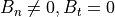
磁場解析結果
解析実行結果は以下に示す.以下に磁束線及び磁場強度の2次元マップと磁場のr依存性を示す.
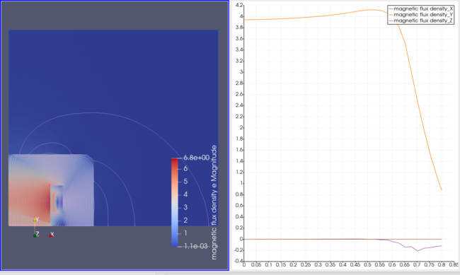
H 型電磁石の磁場強度は約 4 (T) であり、意図した程度の磁場強度が出力されている.
また、Elmer内部で内挿された磁場の軸方向成分を次に示す. paraviewにおけるプロットと一致している.
SaveLine を使用する際の注意点としては、あくまで、内部情報は線形内挿によって得られている点 ( 高精度ではない )と、Elmer からの出力時には、PolyLine として定義した線分に則ってデータが格納されてない点である.前者はそういう仕様なので我慢するしかなく(もしくは自作)、後者の問題はデータ出力後、プロット前にソートする必要がある.単純に、
index = np.argsort( xAxis )
xAxis = xAxis[index]
yAxis = yAxis[index]
でよい.