円環コイル電流が作る磁場
円環コイル電流が作る磁場の解析結果を以下に示す. 問題設定、及び、Elmer入力ファイルは、Elmer のテスト問題、及び、Elmer Discussion Forum のファイルを参考にしている.
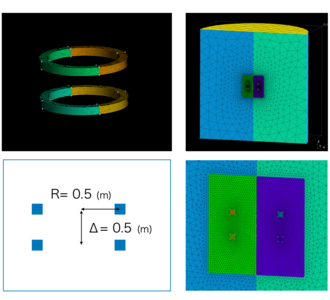
問題設定 / メッシュ
半径
 の円環状のコイルを考え、内部を一様に流れる直流電流が作る磁場を考える.
計算領域は、円筒の計算空間を考え、とある半径
 で電磁ポテンシャルは Dirichlet 条件を課す.
電流として、片側 1.0 A の電流を与える.半径 0.5 m のコイルを距離 0.5 m だけ離して設置する.いわゆる Helmhortz コイルである.
円環コイル電流モデル ( 1/2モデル ver. )のメッシュ生成 プログラム
まずは、円筒の空気領域のうち半分の領域を考え、対称条件を課して計算する.
gmsh-API pythonを利用した円環コイル電流用メッシュの生成プログラム. 自分で作成した円筒形状生成用関数を内部で利用している.
  1import numpy as np
  2import os, sys
  3import gmsh
  4
  5gmshlib = os.environ["gmshLibraryPath"]
  6sys.path.append( gmshlib )
  7
  8import generate__fanShape    as fan
  9import generate__sectorShape as sct
 10
 11# ------------------------------------------------- #
 12# --- [1] initialization of the gmsh            --- #
 13# ------------------------------------------------- #
 14gmsh.initialize()
 15gmsh.option.setNumber( "General.Terminal", 1 )
 16gmsh.model.add( "model" )
 17
 18
 19# ------------------------------------------------- #
 20# --- [2] initialize settings                   --- #
 21# ------------------------------------------------- #
 22ptsDim , lineDim , surfDim , voluDim  =  0,  1,  2,  3
 23pts    , line    , surf    , volu     = {}, {}, {}, {}
 24ptsPhys, linePhys, surfPhys, voluPhys = {}, {}, {}, {}
 25lc                                    = 10.0
 26x_, y_, z_, lc_, tag_                 = 0, 1, 2, 3, 4
 27
 28
 29# ------------------------------------------------- #
 30# --- [3] Modeling                              --- #
 31# ------------------------------------------------- #
 32
 33lc_coil        =   0.02
 34lc_roi         =   0.05
 35lc_sim         =   1.0
 36
 37simBoundary__r = 5.0
 38simBoundary__z = 5.0
 39roiBoundary__r = 1.0
 40roiBoundary__z = 1.0
 41
 42rCoil1         =  0.45
 43rCoil2         =  0.55
 44
 45th1            =   0.0
 46th2            = 180.0
 47gap            =  0.20
 48hCoil          =  0.10
 49
 50ret1 = fan.generate__fanShape   ( lc=lc_coil, r1=rCoil1, r2=rCoil2, th1=th1, th2=th2, \
 51                                  zoffset=+gap, height=+hCoil, defineVolu=True )
 52ret2 = fan.generate__fanShape   ( lc=lc_coil, r1=rCoil1, r2=rCoil2, th1=th1, th2=th2, \
 53                                  zoffset=-gap, height=-hCoil, defineVolu=True )
 54
 55ret3 = fan.generate__fanShape   ( lc=lc_roi , r1=0.0, r2=roiBoundary__r, th1=th1, th2=th2, \
 56                                  zoffset=-roiBoundary__z, height=2.0*roiBoundary__z, \
 57                                  defineVolu=True )
 58ret4 = fan.generate__fanShape   ( lc=lc_sim , r1=0.0, r2=simBoundary__r, th1=th1, th2=th2, \
 59                                  zoffset=-simBoundary__z, height=2.0*simBoundary__z, \
 60                                  defineVolu=True )
 61gmsh.model.occ.addPoint( 0.0, 0.0, 0.0, meshSize=lc_coil  )
 62gmsh.model.occ.removeAllDuplicates()
 63
 64volu["coil_upr"] = ret1["volu"]["fan"]
 65volu["coil_lwr"] = ret2["volu"]["fan"]
 66volu["roi_Area"] = ret3["volu"]["fan"]
 67volu["sim_Area"] = ret4["volu"]["fan"]
 68
 69surf["coil_upr_in"]   = 4
 70surf["coil_upr_out"]  = 7
 71surf["coil_lwr_in"]   = 12
 72surf["coil_lwr_out"]  = 15
 73
 74surf["sim_bot"]       = 24
 75surf["sim_side1"]     = 25
 76surf["sim_top"]       = 26
 77surf["sim_side2"]     = 28
 78
 79surf["x=0_roi1"]      = 17
 80surf["x=0_roi2"]      = 18
 81surf["x=0_sim1"]      = 23
 82surf["x=0_sim2"]      = 27
 83
 84
 85# ------------------------------------------------- #
 86# --- [4] Physical Grouping                     --- #
 87# ------------------------------------------------- #
 88gmsh.model.occ.synchronize()
 89voluPhys["coil_upr"] = gmsh.model.addPhysicalGroup( voluDim, [ volu["coil_upr"] ], tag=301 )
 90voluPhys["coil_lwr"] = gmsh.model.addPhysicalGroup( voluDim, [ volu["coil_lwr"] ], tag=302 )
 91voluPhys["roi_Area"] = gmsh.model.addPhysicalGroup( voluDim, [ volu["roi_Area"] ], tag=303 )
 92voluPhys["sim_Area"] = gmsh.model.addPhysicalGroup( voluDim, [ volu["sim_Area"] ], tag=304 )
 93
 94
 95surfPhys["sim_bot"]      = gmsh.model.addPhysicalGroup( surfDim, [ surf["sim_bot"     ] ], tag=201 )
 96surfPhys["sim_top"]      = gmsh.model.addPhysicalGroup( surfDim, [ surf["sim_top"     ] ], tag=202 )
 97surfPhys["sim_side1"]    = gmsh.model.addPhysicalGroup( surfDim, [ surf["sim_side1"   ] ], tag=203 )
 98surfPhys["sim_side2"]    = gmsh.model.addPhysicalGroup( surfDim, [ surf["sim_side2"   ] ], tag=204 )
 99
100surfPhys["coil_upr_in"]  = gmsh.model.addPhysicalGroup( surfDim, [ surf["coil_upr_in" ] ], tag=205 )
101surfPhys["coil_upr_out"] = gmsh.model.addPhysicalGroup( surfDim, [ surf["coil_upr_out"] ], tag=206 )
102surfPhys["coil_lwr_in"]  = gmsh.model.addPhysicalGroup( surfDim, [ surf["coil_lwr_in" ] ], tag=207 )
103surfPhys["coil_lwr_out"] = gmsh.model.addPhysicalGroup( surfDim, [ surf["coil_lwr_out"] ], tag=208 )
104
105surfPhys["x=0_roi1"]     = gmsh.model.addPhysicalGroup( surfDim, [ surf["x=0_roi1"    ] ], tag=209 )
106surfPhys["x=0_roi2"]     = gmsh.model.addPhysicalGroup( surfDim, [ surf["x=0_roi2"    ] ], tag=210 )
107surfPhys["x=0_sim1"]     = gmsh.model.addPhysicalGroup( surfDim, [ surf["x=0_sim1"    ] ], tag=211 )
108surfPhys["x=0_sim2"]     = gmsh.model.addPhysicalGroup( surfDim, [ surf["x=0_sim2"    ] ], tag=212 )
109
110
111# ------------------------------------------------- #
112# --- [2] post process                          --- #
113# ------------------------------------------------- #
114gmsh.model.occ.synchronize()
115gmsh.model.mesh.generate(3)
116gmsh.write( "model.geo_unrolled" )
117gmsh.write( "model.msh" )
118gmsh.finalize()
119
生成用プログラムの実行は、以下の通り.
$ cd msh_half/
$ python main.py
$ ElmerGrid 14 2 model.msh
$ cd ../
$ mv msh_half/model ./
ElmerGridによって、( 14 : gmshの.mshファイル、 2 : ElmerMeshファイル4つを含んだディレクトリ )へと変換している.model.header / model.element / model.node / model.boundary が生成される.
円環コイル電流が作る磁場のElmer入力ファイル
以下にElmer入力ファイルのサンプルを示す.
  1! ========================================================= !
  2! ===  circular coil half                               === !
  3! ========================================================= !
  4
  5! ------------------------------------------------- !
  6! --- [1] Global Simulation Settings            --- !
  7! ------------------------------------------------- !
  8
  9CHECK KEYWORDS "Warn"
 10
 11Header
 12  Mesh DB "." "model_half"
 13  Include Path ""
 14  Results Directory ""
 15End
 16
 17Simulation
 18  coordinate system           = "Cartesian"
 19  Coordinate Mapping(3)       = 1 2 3
 20
 21  Simulation Type             = "Steady State"
 22  Steady State Max Iterations = 1
 23
 24  Solver Input File           = "circular_coil.sif"
 25  Output File                 = "circular_coil.dat"
 26  Post File                   = "circular_coil.vtu"
 27End
 28
 29Constants
 30  Permeability of Vacuum      = 1.2566e-06
 31End
 32
 33! ------------------------------------------------- !
 34! --- [2] Body & Material Settings              --- !
 35! ------------------------------------------------- !
 36
 37Body 1
 38  Target Bodies(2)       = 301 302
 39  Name                   = "coil"
 40
 41  Equation               = 1
 42  Material               = 1
 43  Body Force             = 1
 44End
 45
 46Body 2
 47  Target Bodies(2)       = 303 304
 48  Name                   = "Air"
 49
 50  Equation               = 2
 51  Material               = 2
 52End
 53
 54
 55Material 1
 56  Name                   = "Metal"
 57  Electric Conductivity  = 5.0e4
 58  Relative Permittivity  = 1.0
 59  Relative Permeability  = 1.0
 60End
 61
 62Material 2
 63  Name                   = "Air"
 64  Electric Conductivity  = 0.0
 65  Relative Permittivity  = 1.0
 66  Relative Permeability  = 1.0
 67End
 68
 69
 70! ------------------------------------------------- !
 71! --- [3] Equation & Solver Settings            --- !
 72! ------------------------------------------------- !
 73
 74Equation 1
 75  Name                   = "MagneticField_in_Coil"
 76  Active Solvers(3)      = 1 2 3
 77End
 78
 79Equation 2
 80  Name                   = "MagneticField_in_Air"
 81  Active Solvers(2)      = 2 3
 82End
 83
 84
 85Solver 1
 86  Equation                            = "CoilSolver"
 87  Procedure                           = "CoilSolver" "CoilSolver"
 88
 89  Linear System Solver                = "Iterative"
 90  Linear System Preconditioning       = "ILU1"
 91  Linear System Max Iterations        = 1000
 92  Linear System Convergence Tolerance = 1e-08
 93  Linear System Iterative Method      = "BiCGStabL"
 94  Linear System Residual Output       = 20
 95  Steady State Convergence Tolerance  = 1e-06
 96  Linear System Symmetric             = True
 97
 98  Desired Coil Current                = Real 2.0
 99  Nonlinear System Consistent Norm    = True
100End
101
102Solver 2
103  Equation                            = "WhitneySolver"
104  Procedure                           = "MagnetoDynamics" "WhitneyAVSolver"
105  Variable                            = String "AV"
106  Variable Dofs                       = 1
107
108  Linear System Solver                = "Iterative"
109  Linear System Iterative Method      = "BiCGStab"
110  Linear System Max Iterations        = 3000
111  Linear System Convergence Tolerance = 1.0e-5
112  Linear System Preconditioning       = "None"
113  Linear System Symmetric             = True
114End
115
116Solver 3
117  Equation                            = "MGDynamicsCalc"
118  Procedure                           = "MagnetoDynamics" "MagnetoDynamicsCalcFields"
119  Potential Variable                  = String "AV"
120
121  Calculate Current Density           = Logical True
122  Calculate Magnetic Field Strength   = Logical True
123
124  Steady State Convergence Tolerance  = 0
125  Linear System Solver                = "Iterative"
126  Linear System Preconditioning       = None
127  Linear System Residual Output       = 0
128  Linear System Max Iterations        = 5000
129  Linear System Iterative Method      = "CG"
130  Linear System Convergence Tolerance = 1.0e-8
131  Linear System Symmetric             = True
132
133  Calculate Nodal Fields              = Logical False
134  Impose Body Force Potential         = Logical True
135  Impose Body Force Current           = Logical True
136  Discontinuous Bodies                = True
137End
138
139
140! ------------------------------------------------- !
141! --- [4] Body Forces / Initial Conditions      --- !
142! ------------------------------------------------- !
143
144Body Force 1
145! -- Give the driving external potential -- !
146  Electric Potential = Equals "CoilPot"
147End
148
149
150! ------------------------------------------------- !
151! --- [5] Boundary Conditions                   --- !
152! ------------------------------------------------- !
153
154Boundary Condition 1
155  Name = "Far Boundary"
156  Target Boundaries(4) = 201 202 203 204
157  AV {e} = 0.0
158End
159
160Boundary Condition 2
161  Name                 = "current in"
162  Target Boundaries(2) = 205 207
163  Coil End             = True
164  AV {e} = 0.0
165End
166
167Boundary Condition 3
168  Name                 = "current out"
169  Target Boundaries(2) = 206 208
170  Coil Start           = True
171  AV {e} = 0.0
172End
173
174Boundary Condition 4
175  Name                 = "x=0 Boundary"
176  Target Boundaries(4) = 209 210 211 212
177  AV {e} = 0.0
178End
円環コイルがつくる磁場計算(1/2モデル)の入力ファイルの要点は以下である.
解いた電磁ポテンシャルから電磁場を計算するために、 MagnetoDynamicsCalcFields を使用する.
磁場計算には WhitneyAVSolver を用いる. これは、電磁ポテンシャルを統一的に解くソルバ.
コイル電流は CoilSolver を使用して計算する. CoilSolver は、要素内部の電流連続の式を解くソルバ.コイル電流はある境界から流入し、別の境界から流出していくことになる.簡易的にコイル電流を生成するために、以下の設定を用いる.
コイル電流の値は、ソルバ内の Desired Coil Current により指定する.電流逆向きにするためには、Coil の Start/End を逆にするか、電流を負として設定する.
Body Force にて、電流源を設定する. Electric Potential として、"CoilPot" を指定する.
Boundary Condition として、 Coil Start / Coil End を指定する.
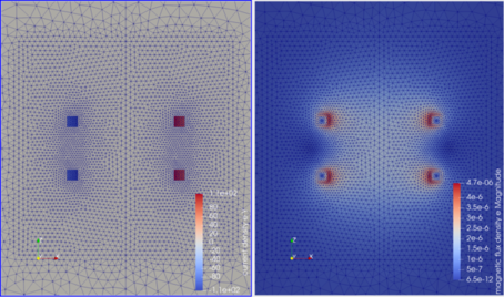
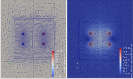
円環コイル電流がつくる磁場の解析結果
解析実行結果は以下に示す.以下に電流密度分布と軸方向の磁束密度を示す.
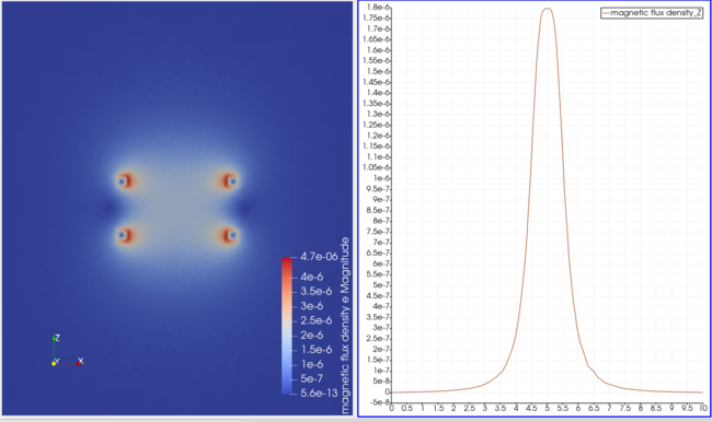
軸方向の磁束密度、及び、 z 軸方向の1次元分布を示す.
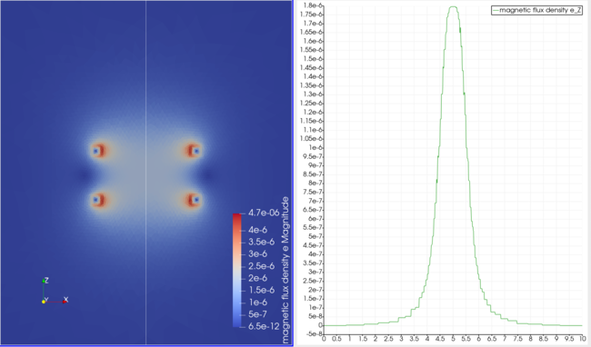
Helmhortz コイルが中心位置につくる磁場は、次のように計算される.
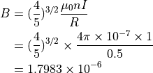
この値は、上記した z 軸方向の1次元分布の値と一致している.
円環コイル電流モデル ( フルモデル ver. )のメッシュ生成 プログラム
次に、円筒の空気領域の全領域を考えたフルモデルの生成プログラムを以下に示す.
  1import numpy as np
  2import os, sys
  3import gmsh
  4
  5gmshlib = os.environ["gmshLibraryPath"]
  6sys.path.append( gmshlib )
  7
  8import generate__fanShape    as fan
  9import generate__sectorShape as sct
 10
 11# ------------------------------------------------- #
 12# --- [1] initialization of the gmsh            --- #
 13# ------------------------------------------------- #
 14gmsh.initialize()
 15gmsh.option.setNumber( "General.Terminal", 1 )
 16gmsh.model.add( "model" )
 17
 18
 19# ------------------------------------------------- #
 20# --- [2] initialize settings                   --- #
 21# ------------------------------------------------- #
 22ptsDim , lineDim , surfDim , voluDim  =  0,  1,  2,  3
 23pts    , line    , surf    , volu     = {}, {}, {}, {}
 24ptsPhys, linePhys, surfPhys, voluPhys = {}, {}, {}, {}
 25lc                                    = 10.0
 26x_, y_, z_, lc_, tag_                 = 0, 1, 2, 3, 4
 27
 28
 29# ------------------------------------------------- #
 30# --- [3] Modeling                              --- #
 31# ------------------------------------------------- #
 32
 33lc_coil        = 0.02
 34lc_roi         = 0.05
 35lc_sim         = 1.00
 36
 37simBoundary__r = 5.0
 38simBoundary__z = 5.0
 39roiBoundary__r = 1.0
 40roiBoundary__z = 1.0
 41
 42rCoil1         = 0.45
 43rCoil2         = 0.55
 44
 45th1            =   0.0
 46th2            = 180.0
 47gap            =  0.20
 48hCoil          =  0.10
 49
 50ret1 = fan.generate__fanShape   ( lc=lc_coil, r1=rCoil1, r2=rCoil2, th1=th1, th2=th2, \
 51                                  zoffset=+gap, height=+hCoil, defineVolu=True, side="+" )
 52ret2 = fan.generate__fanShape   ( lc=lc_coil, r1=rCoil1, r2=rCoil2, th1=th1, th2=th2, \
 53                                  zoffset=+gap, height=+hCoil, defineVolu=True, side="-" )
 54ret3 = fan.generate__fanShape   ( lc=lc_coil, r1=rCoil1, r2=rCoil2, th1=th1, th2=th2, \
 55                                  zoffset=-gap, height=-hCoil, defineVolu=True, side="+" )
 56ret4 = fan.generate__fanShape   ( lc=lc_coil, r1=rCoil1, r2=rCoil2, th1=th1, th2=th2, \
 57                                  zoffset=-gap, height=-hCoil, defineVolu=True, side="-" )
 58
 59ret5 = fan.generate__fanShape   ( lc=lc_roi , r1=0.0, r2=roiBoundary__r, th1=th1, th2=th2, \
 60                                  zoffset=-roiBoundary__z, height=2.0*roiBoundary__z, \
 61                                  defineVolu=True, side="+" )
 62ret6 = fan.generate__fanShape   ( lc=lc_roi , r1=0.0, r2=roiBoundary__r, th1=th1, th2=th2, \
 63                                  zoffset=-roiBoundary__z, height=2.0*roiBoundary__z, \
 64                                  defineVolu=True, side="-" )
 65ret7 = fan.generate__fanShape   ( lc=lc_sim , r1=0.0, r2=simBoundary__r, th1=th1, th2=th2, \
 66                                  zoffset=-simBoundary__z, height=2.0*simBoundary__z, \
 67                                  defineVolu=True, side="+" )
 68ret8 = fan.generate__fanShape   ( lc=lc_sim , r1=0.0, r2=simBoundary__r, th1=th1, th2=th2, \
 69                                  zoffset=-simBoundary__z, height=2.0*simBoundary__z, \
 70                                  defineVolu=True, side="-" )
 71
 72gmsh.model.occ.addPoint( 0.0, 0.0, 0.0, meshSize=lc_coil )
 73gmsh.model.occ.removeAllDuplicates()
 74
 75volu["coil_upr1"] = ret1["volu"]["fan"]
 76volu["coil_upr2"] = ret2["volu"]["fan"]
 77volu["coil_lwr1"] = ret3["volu"]["fan"]
 78volu["coil_lwr2"] = ret4["volu"]["fan"]
 79volu["roi_Area1"] = ret5["volu"]["fan"]
 80volu["roi_Area2"] = ret6["volu"]["fan"]
 81volu["sim_Area1"] = ret7["volu"]["fan"]
 82volu["sim_Area2"] = ret8["volu"]["fan"]
 83
 84surf["sim_top1"]  = 38
 85surf["sim_bot1"]  = 36
 86surf["sim_bot2"]  = 41
 87surf["sim_top2"]  = 43
 88surf["sim_side1"] = 37
 89surf["sim_side2"] = 40
 90surf["sim_side3"] = 44
 91surf["sim_side4"] = 42
 92
 93surf["coil_upr_in"]   = 45
 94surf["coil_upr_out"]  = 46
 95surf["coil_lwr_in"]   = 47
 96surf["coil_lwr_out"]  = 48
 97
 98# ------------------------------------------------- #
 99# --- [4] Physical Grouping                     --- #
100# ------------------------------------------------- #
101gmsh.model.occ.synchronize()
102voluPhys["coil_upr1"] = gmsh.model.addPhysicalGroup( voluDim, [ volu["coil_upr1"] ], tag=301 )
103voluPhys["coil_upr2"] = gmsh.model.addPhysicalGroup( voluDim, [ volu["coil_upr2"] ], tag=302 )
104voluPhys["coil_lwr1"] = gmsh.model.addPhysicalGroup( voluDim, [ volu["coil_lwr1"] ], tag=303 )
105voluPhys["coil_lwr2"] = gmsh.model.addPhysicalGroup( voluDim, [ volu["coil_lwr2"] ], tag=304 )
106voluPhys["roi_Area1"] = gmsh.model.addPhysicalGroup( voluDim, [ volu["roi_Area1"] ], tag=305 )
107voluPhys["roi_Area2"] = gmsh.model.addPhysicalGroup( voluDim, [ volu["roi_Area2"] ], tag=306 )
108voluPhys["sim_Area1"] = gmsh.model.addPhysicalGroup( voluDim, [ volu["sim_Area1"] ], tag=307 )
109voluPhys["sim_Area2"] = gmsh.model.addPhysicalGroup( voluDim, [ volu["sim_Area2"] ], tag=308 )
110
111surfPhys["sim_bot1"]  = gmsh.model.addPhysicalGroup( surfDim, [ surf["sim_bot1" ] ], tag=201 )
112surfPhys["sim_bot2"]  = gmsh.model.addPhysicalGroup( surfDim, [ surf["sim_bot2" ] ], tag=202 )
113surfPhys["sim_top1"]  = gmsh.model.addPhysicalGroup( surfDim, [ surf["sim_top1" ] ], tag=203 )
114surfPhys["sim_top2"]  = gmsh.model.addPhysicalGroup( surfDim, [ surf["sim_top2" ] ], tag=204 )
115surfPhys["sim_side1"] = gmsh.model.addPhysicalGroup( surfDim, [ surf["sim_side1"] ], tag=205 )
116surfPhys["sim_side2"] = gmsh.model.addPhysicalGroup( surfDim, [ surf["sim_side2"] ], tag=206 )
117surfPhys["sim_side3"] = gmsh.model.addPhysicalGroup( surfDim, [ surf["sim_side3"] ], tag=207 )
118surfPhys["sim_side4"] = gmsh.model.addPhysicalGroup( surfDim, [ surf["sim_side4"] ], tag=208 )
119
120surfPhys["coil_upr_in"]  = gmsh.model.addPhysicalGroup( surfDim, [ surf["coil_upr_in" ] ], tag=209 )
121surfPhys["coil_upr_out"] = gmsh.model.addPhysicalGroup( surfDim, [ surf["coil_upr_out"] ], tag=210 )
122surfPhys["coil_lwr_in"]  = gmsh.model.addPhysicalGroup( surfDim, [ surf["coil_lwr_in" ] ], tag=211 )
123surfPhys["coil_lwr_out"] = gmsh.model.addPhysicalGroup( surfDim, [ surf["coil_lwr_out"] ], tag=212 )
124
125# ------------------------------------------------- #
126# --- [2] post process                          --- #
127# ------------------------------------------------- #
128gmsh.model.occ.synchronize()
129gmsh.model.mesh.generate(3)
130gmsh.write( "model.geo_unrolled" )
131gmsh.write( "model.msh" )
132gmsh.finalize()
133
円環コイル電流が作る磁場のElmer入力ファイル (フルモデル用)
以下にフルモデル用のElmer入力ファイルのサンプルを示す.
  1! ========================================================= !
  2! ===  circular coil half                               === !
  3! ========================================================= !
  4
  5! ------------------------------------------------- !
  6! --- [1] Global Simulation Settings            --- !
  7! ------------------------------------------------- !
  8
  9CHECK KEYWORDS "Warn"
 10
 11Header
 12  Mesh DB "." "model_full"
 13  Include Path ""
 14  Results Directory ""
 15End
 16
 17Simulation
 18  coordinate system           = "Cartesian"
 19  Coordinate Mapping(3)       = 1 2 3
 20
 21  Simulation Type             = "Steady State"
 22  Steady State Max Iterations = 1
 23
 24  Solver Input File           = "circular_coil.sif"
 25  Output File                 = "circular_coil.dat"
 26  Post File                   = "circular_coil.vtu"
 27End
 28
 29
 30Constants
 31  Permeability of Vacuum = 1.2566e-06
 32End
 33
 34
 35! ------------------------------------------------- !
 36! --- [2] Body & Material Settings              --- !
 37! ------------------------------------------------- !
 38
 39Body 1
 40  Target Bodies(2) = 301 302
 41  Name             = "coil1"
 42
 43  Equation         = 1
 44  Material         = 1
 45  Body Force       = 1
 46End
 47
 48Body 2
 49  Target Bodies(2) = 303 304
 50  Name             = "coil2"
 51
 52  Equation         = 1
 53  Material         = 1
 54  Body Force       = 1
 55End
 56
 57Body 3
 58  Target Bodies(4) = 305 306 307 308
 59  Name             = "Air"
 60
 61  Equation         = 2
 62  Material         = 2
 63End
 64
 65
 66Material 1
 67  Name                  = "Metal"
 68  Electric Conductivity = 5.0e4
 69  Relative Permittivity = 1.0
 70  Relative Permeability = 1.0
 71End
 72
 73Material 2
 74  Name                  = "Air"
 75  Electric Conductivity = 0.0
 76  Relative Permittivity = 1.0
 77  Relative Permeability = 1.0
 78End
 79
 80
 81Component 1
 82  Name                    = "Coil1"
 83  Coil Type               = "test"
 84  Master Bodies(1)        = 1
 85  ! Desired Current Density = Real -1.0e3
 86  Desired Coil Current    = +1.0
 87End
 88
 89Component 2
 90  Name                    = "Coil2"
 91  Coil Type               = "test"
 92  Master Bodies(1)        = 2
 93  ! Desired Current Density = Real 1.0e3
 94  Desired Coil Current    = -1.0
 95End
 96
 97
 98! ------------------------------------------------- !
 99! --- [3] Equation & Solver Settings            --- !
100! ------------------------------------------------- !
101
102Equation 1
103  Name              = "MagneticField_in_Coil"
104  Active Solvers(3) = 1 2 3
105End
106
107Equation 2
108  Name              = "MagneticField_in_Air"
109  Active Solvers(2) = 2 3
110End
111
112
113Solver 1
114  Equation                            = "CoilSolver"
115  Procedure                           = "CoilSolver" "CoilSolver"
116
117  Linear System Solver                = "Iterative"
118  Linear System Preconditioning       = "ILU1"
119  Linear System Max Iterations        = 1000
120  Linear System Convergence Tolerance = 1e-08
121  Linear System Iterative Method      = "BiCGStabL"
122  Linear System Residual Output       = 20
123  Steady State Convergence Tolerance  = 1e-06
124
125  Optimize Bandwidth                  = True
126  Nonlinear System Consistent Norm    = True
127  Coil Closed                         = Logical True
128  Narrow Interface                    = Logical False
129
130  Normalize Coil Current              = Logical True
131  Save Coil Set                       = Logical True
132  Save Coil Index                     = Logical True
133  Calculate Elemental Fields          = Logical True
134End
135
136Solver 2
137  Equation                            = "WhitneySolver"
138  Variable                            = "AV"
139  Variable Dofs                       = 1
140  Procedure                           = "MagnetoDynamics" "WhitneyAVSolver"
141
142  Linear System Solver                = "Iterative"
143  Linear System Iterative Method      = "BiCGStab"
144  Linear System Max Iterations        = 3000
145  Linear System Convergence Tolerance = 1.0e-5
146  Linear System Preconditioning       = "None"
147  Linear System Symmetric             = True
148End
149
150Solver 3
151  Equation                            = "MGDynamicsCalc"
152  Procedure                           = "MagnetoDynamics" "MagnetoDynamicsCalcFields"
153  Potential Variable                  = String "AV"
154
155  Calculate Current Density           = Logical True
156  Calculate Electric Field            = Logical False
157  Calculate Magnetic Field Strength   = Logical True
158  Calculate Joule Heating             = Logical False
159
160  Steady State Convergence Tolerance  = 0
161  Linear System Solver                = "Iterative"
162  Linear System Preconditioning       = None
163  Linear System Residual Output       = 0
164  Linear System Max Iterations        = 5000
165  Linear System Iterative Method      = "CG"
166  Linear System Convergence Tolerance = 1.0e-8
167  Linear System Symmetric             = True
168
169  Nonlinear System Consistent Norm    = Logical True
170  Discontinuous Bodies                = True
171End
172
173
174! ------------------------------------------------- !
175! --- [4] Body Forces / Initial Conditions      --- !
176! ------------------------------------------------- !
177
178Body Force 1
179  Name              = "CoilCurrentSource"
180  Current Density 1 = Equals "CoilCurrent e 1"
181  Current Density 2 = Equals "CoilCurrent e 2"
182  Current Density 3 = Equals "CoilCurrent e 3"
183End
184
185
186! ------------------------------------------------- !
187! --- [5] Boundary Conditions                   --- !
188! ------------------------------------------------- !
189
190Boundary Condition 1
191  Name = "Far Boundary"
192  Target Boundaries(8) = 201 202 203 204 205 206 207 208
193  AV {e}               = 0.0
194End
195
円環コイルがつくる磁場計算(フルモデル)の入力ファイルの要点は以下である.
1/2モデルと同様に、"WhitneyAVSolver", "MagnetoDynamicsCalcFields", "CoilSolver" を解く.
1/2モデルと異なり、フルモデルではループ電流となるため、 CoilSolver における電流の流出入がない.そこで、電流路に2枚の微小距離を離しておいた仮想的な境界面を用意し、2枚の境界面の間にポテンシャルを設定する.微小距離空隙以外の領域(長い流路側)で電流を流す.これを2つ用意してやることでループ電流をつくるらしい.これを用いるために次の設定を用いる.
Body 1 / Body 2 とコイル毎にBody指定を分け、さらに 0次元量としての電源を定義するために、 Component を各 Body に紐付けて定義する.Component 毎に Desired Coil Current を指定しておく.
CoilSolver 内に、 Coil Closed 及び、 Calculate Elemental Fields を True とする.
他、 上の戦略で電流計算するためには、 Narrow Interface を True とする、 コイル情報を示すために、 Set Coil Index , Set Coil Set を True とする. ( False でも構わない ).
Body Force として、Current Density 1,2,3 を定義する.
上記により、ループ電流を定義し、磁場を計算する.
円環コイル電流がつくる磁場の解析結果 ( フルモデル ver. )
解析実行結果は以下に示す.以下に電流密度分布と軸方向の磁束密度を示す.
軸方向の磁束密度、及び、 z 軸方向の1次元分布を示す.
フルモデルでも、 Helmhortz コイルのつくる磁場の理論値と一致する.