線電流が作る磁場¶

直線電流が作る磁場の解析結果を以下に示す．問題設定、及び、Elmer入力ファイルは、Elmer のテスト問題を参考にしている．

問題設定 / メッシュ¶

半径 $R=R_a$ の円筒状導線を一様に流れる直流電流が作る磁場を考える．
計算領域は、円筒の計算空間を考え、とある半径 $R=R_A$ で電磁ポテンシャルは Dirichlet 条件を課す．
電流として、理想電流 1.0 A を与える．

線電流モデルのメッシュ生成用 gmsh-API python プログラム¶

gmsh-API pythonを利用した片持ち梁モデルの生成プログラム．自分で作成した箱生成用関数を内部で利用している．

線電流モデルのメッシュ生成用 gmsh-API python プログラム¶

import numpy as np
import os, sys
import gmsh

gmshlib = os.environ["gmshLibraryPath"]
sys.path.append( gmshlib )
import generate__quadShape as qua
import generate__cylinder  as cyl

# ------------------------------------------------- #
# --- [1] initialization of the gmsh            --- #
# ------------------------------------------------- #
gmsh.initialize()
gmsh.option.setNumber( "General.Terminal", 1 )
gmsh.model.add( "model" )

# ------------------------------------------------- #
# --- [2] initialize settings                   --- #
# ------------------------------------------------- #
ptsDim , lineDim , surfDim , voluDim  =  0,  1,  2,  3
pts    , line    , surf    , volu     = {}, {}, {}, {}
ptsPhys, linePhys, surfPhys, voluPhys = {}, {}, {}, {}
lc                                    = 0.2
x_, y_, z_, lc_, tag_                 = 0, 1, 2, 3, 4

# ------------------------------------------------- #
# --- [3] Modeling                              --- #
# ------------------------------------------------- #

zLeng   =   5.0
wire_r  =   0.3
sim__r  =   3.0

xc      = [    0.0,    0.0,   0.0 ]
delta   = [    0.0,    0.0, zLeng ]

lc_sim  = 0.50
lc_wire = 0.05

ret          = cyl.generate__cylinder ( lc=lc_sim, xc=xc, radius=sim__r, \
                                        defineVolu=True, extrude_delta=delta )
volu["Air"]  = ret["volu"]["cylinder"]

ret          = cyl.generate__cylinder ( lc=lc_wire, xc=xc, radius=wire_r, \
                                        defineVolu=True, extrude_delta=delta )
volu["wire"] = ret["volu"]["cylinder"]
gmsh.model.occ.removeAllDuplicates()

volu["wire"]     = 2
volu["Air"]      = 3

surf["wireIn"]   = 4
surf["wireOut"]  = 6
surf["wireSide"] = 5
surf["AirIn"]    = 8
surf["AirOut"]   = 9
surf["AirSide"]  = 7

# ------------------------------------------------- #
# --- [4] Physical Grouping                     --- #
# ------------------------------------------------- #
gmsh.model.occ.synchronize()
surfPhys["wireIn"]   = gmsh.model.addPhysicalGroup( surfDim, [ surf["wireIn"] ]  , tag=201 )
surfPhys["wireSide"] = gmsh.model.addPhysicalGroup( surfDim, [ surf["wireSide"] ], tag=202 )
surfPhys["wireOut"]  = gmsh.model.addPhysicalGroup( surfDim, [ surf["wireOut"] ] , tag=203 )
surfPhys["AirIn"]    = gmsh.model.addPhysicalGroup( surfDim, [ surf["AirIn"] ]   , tag=204 )
surfPhys["AirSide"]  = gmsh.model.addPhysicalGroup( surfDim, [ surf["AirSide"] ] , tag=205 )
surfPhys["AirOut"]   = gmsh.model.addPhysicalGroup( surfDim, [ surf["AirOut"] ]  , tag=206 )

voluPhys["wire"]     = gmsh.model.addPhysicalGroup( voluDim, [ volu["wire"] ]    , tag=301 )
voluPhys["Air"]      = gmsh.model.addPhysicalGroup( voluDim, [ volu["Air"] ]     , tag=302 )


# ------------------------------------------------- #
# --- [2] post process                          --- #
# ------------------------------------------------- #
gmsh.model.occ.synchronize()
gmsh.model.mesh.generate(3)
gmsh.write( "model.geo_unrolled" )
gmsh.write( "model.msh" )
gmsh.finalize()

生成用プログラムの実行は、以下の通り．

モデル生成¶

$ cd msh/
$ python model.py
$ ElmerGrid 14 2 model.msh
$ cd ../
$ mv msh/model ./

ElmerGridによって、( 14 : gmshの.mshファイル、 2 : ElmerMeshファイル4つを含んだディレクトリ )へと変換している．model.header / model.element / model.node / model.boundary が生成される．

線電流が作る磁場のElmer入力ファイル¶

以下にElmer入力ファイルのサンプルを示す．

線電流がつくる磁場の Elmer 入力ファイル ( line_current.sif )¶

CHECK KEYWORDS "Warn"

Header
  Mesh DB "." "model"
  Include Path ""
  Results Directory ""
End

Simulation
  coordinate system           = "Cartesian"

  Simulation Type             = "Steady State"
  Steady State Max Iterations = 1
  
  Solver Input File           = "line_current.sif"
  Output File                 = "results/line_current.dat"
  Post File                   = "line_current.vtu"
End


Constants
End

Body 1
  Target Bodies(1) = 301
  Name             = "Conductor"

  Equation   = 1
  Material   = 1
  Body Force = 1
End

Body 2
  Target Bodies(1) = 302
  Name             = "Air"

  Equation   = 1
  Material   = 2
End


Material 1
  Name                  = "Conductor"
  Relative Permittivity = 1.0
  Relative Permeability = 1.0
  Electric Conductivity = 5.80e7
End

Material 2
  Name                  = "Air"
  Relative Permittivity = 1.0
  Relative Permeability = 1.0
  Electric Conductivity = 0.0
End


Equation 1
  Name              = "Magnetic Field Equations for Conductor"
  Active Solvers(3) = 1 2 3
End


Equation 2
  Name              = "Magnetic Field Equations for Air"
  Active Solvers(2) = 2 3
End


Solver 1
  Equation                            = "CoilSolver"
  Procedure                           = "CoilSolver" "CoilSolver"

  Linear System Solver                = "Iterative"
  Linear System Preconditioning       = "ILU1"
  Linear System Max Iterations        = 1000
  Linear System Convergence Tolerance = 1e-10
  Linear System Iterative Method      = BiCGStabL
  Linear System Residual Output       = 20
  Steady State Convergence Tolerance  = 1e-06

  Desired Coil Current                = Real 1.0
  Nonlinear System Consistent Norm    = True
End

Solver 2
  Equation                            = "AV"
  Procedure                           = "MagnetoDynamics" "WhitneyAVSolver"

  Linear System Symmetric             = True
  Linear System Solver                = "Iterative"
  Linear System Preconditioning       = None
  Linear System Residual Output       = 10
  Linear System Max Iterations        = 1000
  Linear System Iterative Method      = GCR
  Linear System Convergence Tolerance = 1.0e-8
  BicgStabl Polynomial Degree         = 4
End

Solver 3
  Equation                = "MGDynamicsCalc"

  Procedure               = "MagnetoDynamics" "MagnetoDynamicsCalcFields"
  Linear System Symmetric = True

  Potential Variable      = String "AV"

  Calculate Current Density           = Logical True
  Calculate Electric Field            = Logical True
  Calculate Magnetic Field Strength   = Logical True
  Calculate Joule Heating             = True

  Steady State Convergence Tolerance  = 0
  Linear System Solver                = "Iterative"
  Linear System Preconditioning       = None
  Linear System Residual Output       = 0
  Linear System Max Iterations        = 5000
  Linear System Iterative Method      = CG
  Linear System Convergence Tolerance = 1.0e-8

  Calculate Nodal Fields              = Logical False
  Impose Body Force Potential         = Logical True
  Impose Body Force Current           = Logical True
  Discontinuous Bodies                = True
End

Solver 4
  Exec Solver               = after all
  Equation                  = "ResultOutput"
  Procedure                 = "ResultOutputSolve" "ResultOutputSolver"
  Output File Name          = wire
  Vtu format                = Logical True
  Discontinuous Bodies      = Logical True
End

Solver 5
  Exec Solver               = after all
  Equation                  = "SaveLine"
  Procedure                 = "SaveData" "SaveLine"
  FileName                  = "bfield_inline.dat"

  Polyline Coordinates(2,3) = -5.0e-3 0.0 5.0e-3 5.0e-3 0.0 5.0e-3
  Polyline Divisions(1)     = 100
End


Body Force 1
! a) Give current density
!  Current Density 1 = Equals "CoilCurrent 1"
!  Current Density 2 = Equals "CoilCurrent 2"
!  Current Density 3 = Equals "CoilCurrent 3"

! b) Give the driving external potential
 Electric Potential = Equals "CoilPot"
End


Boundary Condition 1
  Name                 = "WireStart"
  Target Boundaries(1) = 201
  Coil Start           = Logical True
  AV {e} 1 = Real 0.0
  AV {e} 2 = Real 0.0
  AV       = Real 0.0
End

Boundary Condition 2
  Name                 = "WireSurface"
  Target Boundaries(1) = 202
End

Boundary Condition 3
  Name                 = "WireEnd"
  Target Boundaries(1) = 203
  Coil End             = Logical True
  AV {e} 1 = Real 0.0
  AV {e} 2 = Real 0.0
  AV       = Real 0.0
End

Boundary Condition 4
  Name                 = "AirStart"
  Target Boundaries(1) = 204
  AV {e} 1 = Real 0.0
  AV {e} 2 = Real 0.0
End


Boundary Condition 5
  Name                 = "AirSurface"
  Target Boundaries(1) = 205
  AV {e} 1 = Real 0.0
  AV {e} 2 = Real 0.0
End

Boundary Condition 6
  Name                 = "AirEnd"
  Target Boundaries(1) = 206
  AV {e} 1 = Real 0.0
  AV {e} 2 = Real 0.0
End

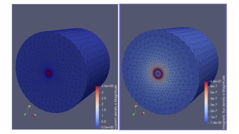
線電流がつくる磁場の解析結果¶

解析実行結果は以下に示す．以下に電流密度分布と磁界強度を示す．

../../../_images/line_current_JDensity_BField.png

以下に磁束密度分布と磁場・電流の径方向1次元分布を示す．

../../../_images/line_current_BFlux_1D.png

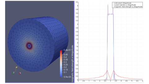
線電流がつくる磁場は、Ampere則、

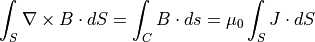
$\int_S \nabla \times B \cdot dS = \int_C B \cdot ds = \mu_0 \int_S J \cdot dS$

を用いて解析的に計算できる．まずは、導体中の磁束密度は、

$2 \pi r B &= \mu_0 J \int_0^r 2 \pi r^{\prime} dr^{\prime} = 2 \pi \mu_0 J [ \dfrac{1}{2}r^{\prime 2 } ]^r_0 \\ B(r) &= \dfrac{ \mu_0 J r }{ 2 }$

導体外側空気領域の磁束密度は、

$2 \pi r B &= \mu_0 J \int_0^a 2 \pi r^{\prime} dr^{\prime} = 2 \pi \mu_0 J [ \dfrac{1}{2}r^{\prime 2} ]^a_0 \\ B(r) &= \dfrac{ \mu_0 J a^2 }{ 2 r } = \dfrac{ \mu_0 I }{ 2 \pi r }$

一次元分布をみると、磁界強度は導体円筒中はrに対して線形に増加し、外側では 1/r で減少しているため、理論解と定性的に一致している．

線電流が作る磁場¶

問題設定 / メッシュ¶

線電流モデルのメッシュ生成用 gmsh-API python プログラム¶

線電流が作る磁場のElmer入力ファイル¶

線電流がつくる磁場の解析結果¶

目次

前のトピックへ

次のトピックへ

このページ