二次電子モニタ測定系の等価回路解析 (1)
背景
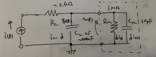
金属片を用いた二次電子モニタを作成
電流源として動作する二次電子モニタに対し、同軸ケーブルでオシロスコープへ接続した場合の観測波形について考えたい.
同軸ケーブル・オシロスコープの等価回路を考えて、観測波形が説明したい.
ポイント
等価回路から導出される一般解は、得られる波形を説明できるか?
等価回路の回路定数を用いて、得られる波形を説明できるか?
振幅
時間構造 ( 周期、時定数 )
オフセット
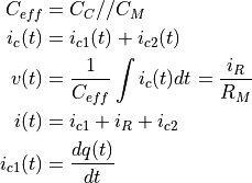
![v(t) &= R_M i_0 \left[ 1 - e^{ - \dfrac{t} {R_M C_{eff}} } \right] \\
i_{c}(t) &= i_0 e^{ - \dfrac{t} {R_M C_{eff}} } \\
q(t) &= R_M C_{eff} i_0 \left[ 1 - e^{ - \dfrac{t} {R_M C_{eff}} } \right] \\](../../../_images/math/4cf18bb92557a68486c05dba6ce24f3bc46a79d2.png)
![v(t) &= R_M i_0 \left[ 1 - e^{ - \dfrac{\tau_1 }{ R_M C_{eff} } } \right] e^{ - \dfrac{t-\tau_1} {R_M C_{eff}} } \\
i_{c}(t) &= i_0 \left[ 1 - e^{ - \dfrac{\tau_1 }{ R_M C_{eff} } } \right] e^{ - \dfrac{t-\tau_1} {R_M C_{eff}} } \\
q(t) &= R_M C_{eff} i_0 \left[ 1 - e^{ - \dfrac{\tau_1 }{ R_M C_{eff} } } \right] e^{ - \dfrac{t-\tau_1} {R_M C_{eff}} } \\](../../../_images/math/f830fcf718a7167f79f8a1eb3815815b779e02a1.png)
信号波形(解析値)
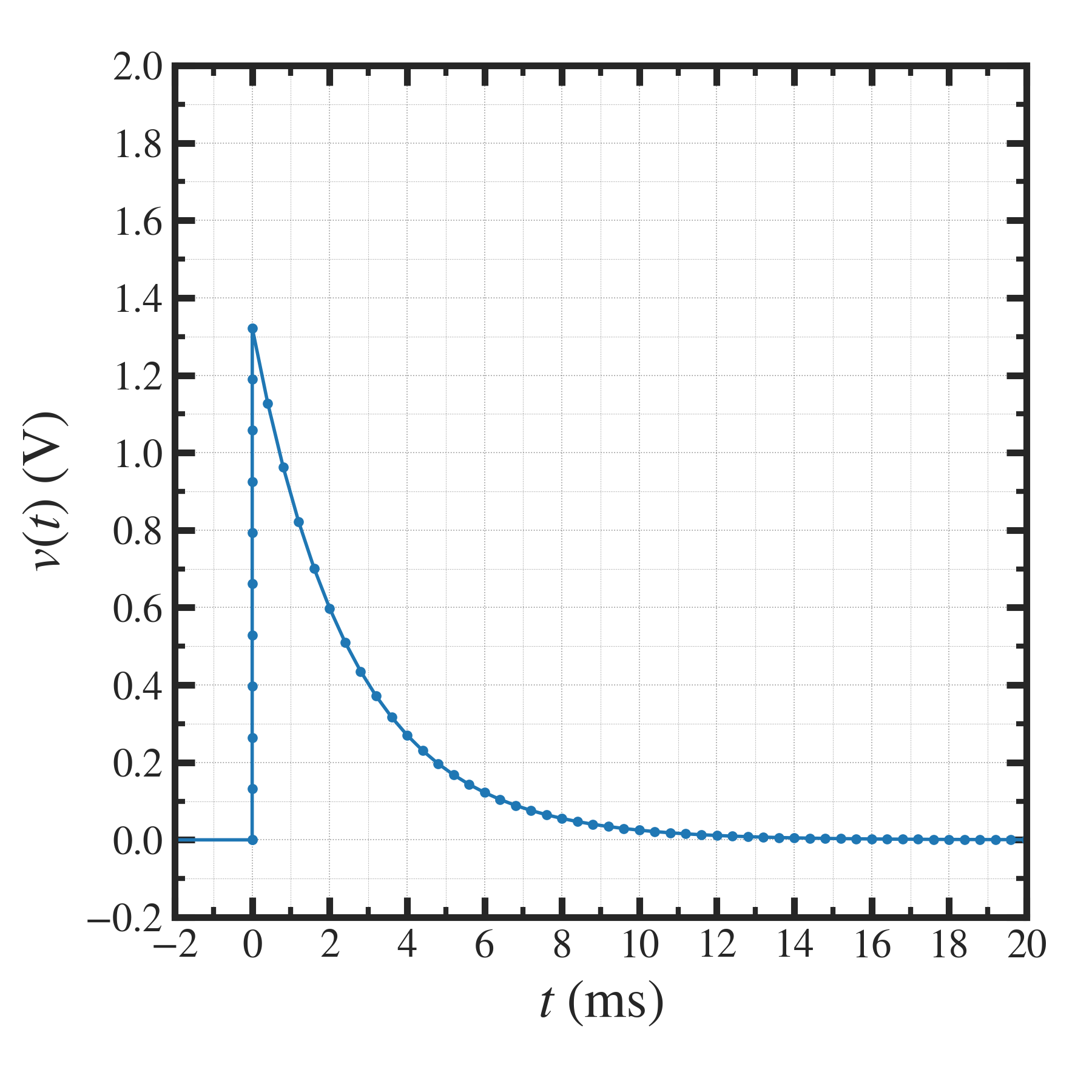
理論信号波形プロット (一般解)
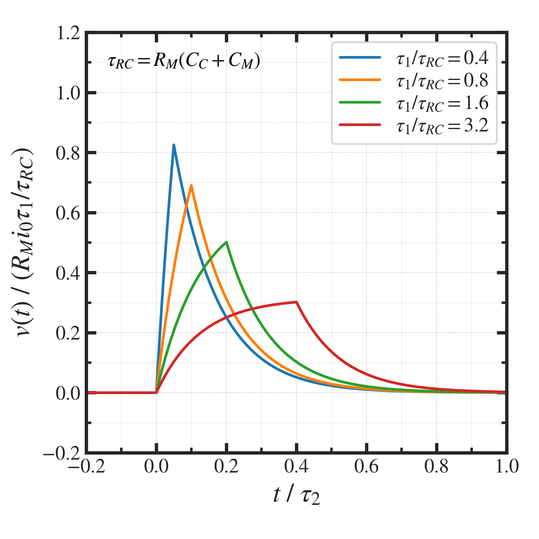
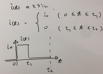
ビームパルス(
 )が、回路の時定数(
  )よりも、十分、短時間であれば、パルス状に瞬時に立ち上がり、そのあと、減衰していく波形となる.(実際に観測されたデータはそのような波形)
図示プログラム
import numpy as np


# ========================================================= #
# ===  SEEmonitor_model_graph.py                        === #
# ========================================================= #

def SEEmonitor_model_graph():

    ms             = 1.e-3
    t_, v_, i_, q_ = 0, 1, 2, 3

    # ------------------------------------------------- #
    # --- [1] def parameters                        --- #
    # ------------------------------------------------- #
    CC          = 8.8e-9
    RC          = 2.5
    CM          = 20.0e-12
    RM          = 1.0e+6
    tau1        = 3.0e-6
    tau2        = 3.3e-3
    tau3        = 20.0e-3
    nT1         = 11
    nT2         = 51
    I_SEE_ave   = 2.0e-6
    tau_beam    = 3.0e-6
    f_Repeat    = 300.0
    duty        = tau_beam * f_Repeat
    I_SEE_pulse = I_SEE_ave / duty
    i0          = I_SEE_pulse
    print( " i0 == {}".format( i0 ) )

    # ------------------------------------------------- #
    # --- [2] calculation                           --- #
    # ------------------------------------------------- #
    tauRC = RM * ( CC + CM )
    t_pre = np.array( [-1e10, 0.0] )
    t1    = ( np.linspace(  0.0, tau1     , nT1 ) )[0:]
    # t2    = ( np.linspace( tau1, tau1+tau2, nT2 ) )[1:]
    t2    = ( np.linspace( tau1, tau3, nT2 ) )[1:]
    qchg  = tauRC * i0 * ( 1.0 - np.exp( - tau1  / tauRC ) )

    v1    = RM    * i0 * ( 1.0 - np.exp( - t1 / tauRC ) )
    i1    =         i0 * (       np.exp( - t1 / tauRC ) )
    q1    = tauRC * i0 * ( 1.0 - np.exp( - t1 / tauRC ) )
    v2    = qchg / (CC+CM) * ( np.exp( - ( t2 - tau1 ) / tauRC ) )
    i2    = qchg / tauRC   * ( np.exp( - ( t2 - tau1 ) / tauRC ) )
    q2    = qchg           * ( np.exp( - ( t2 - tau1 ) / tauRC ) )

    v_pre = np.array( [0.0,0.0] )
    i_pre = np.array( [0.0,0.0] )
    q_pre = np.array( [0.0,0.0] )

    time  = np.reshape( np.concatenate( [t_pre,t1,t2] ), [-1,1] )
    vt    = np.reshape( np.concatenate( [v_pre,v1,v2] ), [-1,1] )
    it    = np.reshape( np.concatenate( [i_pre,i1,i2] ), [-1,1] )
    qt    = np.reshape( np.concatenate( [q_pre,q1,q2] ), [-1,1] )
    Data  = np.concatenate( [time,vt,it,qt], axis=1 )
    print( Data.shape )

    # ------------------------------------------------- #
    # --- [3] save data in a file                   --- #
    # ------------------------------------------------- #
    import nkUtilities.save__pointFile as spf
    outFile   = "dat/SEEmonitor_model_graph.dat"
    spf.save__pointFile( outFile=outFile, Data=Data, names=["t","v(t)", "i(t)", "q(t)"] )

    # ------------------------------------------------- #
    # --- [4] display in a file                     --- #
    # ------------------------------------------------- #
    import nkUtilities.plot1D         as pl1
    import nkUtilities.load__config   as lcf
    import nkUtilities.configSettings as cfs
    x_,y_                    = 0, 1
    pngFile                  = "png/SEEmonitor_model_graph_v_vs_time.png"
    config                   = lcf.load__config()
    config                   = cfs.configSettings( configType="plot.def", config=config )
    config["FigSize"]        = (4.5,4.5)
    config["plt_position"]   = [ 0.16, 0.16, 0.94, 0.94 ]
    config["plt_xAutoRange"] = False
    config["plt_yAutoRange"] = False
    config["plt_xRange"]     = [ -2.0, +20.0 ]
    config["plt_yRange"]     = [ -0.2, +2.0  ]
    config["xMajor_Nticks"]  = 12
    config["yMajor_Nticks"]  = 12
    config["plt_marker"]     = "o"
    config["plt_markersize"] = 2.0
    config["plt_linestyle"]  = "-"
    config["plt_linewidth"]  = 1.0
    config["xTitle"]         = "$t \ \mathrm{(ms)}$"
    config["yTitle"]         = "$v(t) \ \mathrm{(V)}$"
    fig     = pl1.plot1D( config=config, pngFile=pngFile )
    fig.add__plot( xAxis=Data[:,t_]/ms, yAxis=Data[:,v_] )
    fig.set__axis()
    fig.save__figure()
    return()


# ========================================================= #
# ===   Execution of Pragram                            === #
# ========================================================= #

if ( __name__=="__main__" ):
    SEEmonitor_model_graph()